When getting started with SPSS, you may initially be confused about how to input your data in such a way that it’s easy to read and will allow you do to do the analyses that you would like to do.

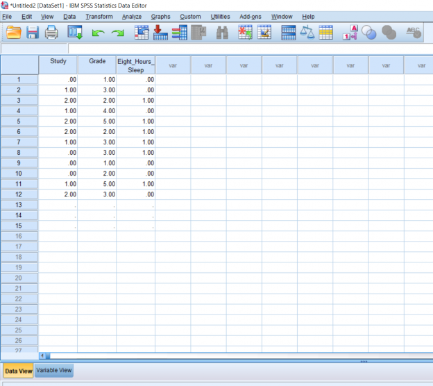
When first opening a new dataset on SPSS, you will be greeted with this blank screen on the Data View tab.

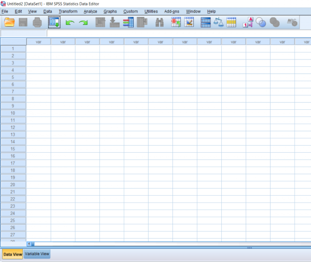
The Data View tab is where you will be inputting the actual data. The way the data should be organized is that all data corresponding to a variable is lined up by column. Data for more than one variable which corresponds to an individual should be organized by row. The picture shows data for three variables organized by column.

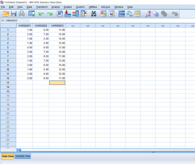
But I want to know what it is I’m looking at; which column corresponds to which variable? This is when you would click on the Variable view tab to name your variables. All you have to do is click on the variable you want to rename and type in the name like an Excel spreadsheet.

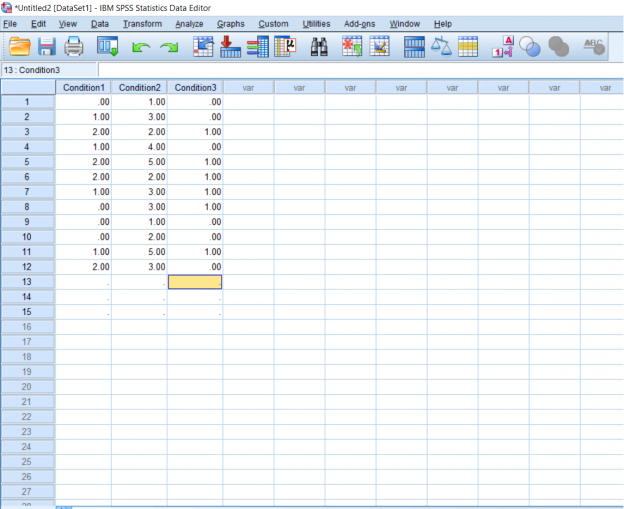
If you’re working with interval or ratio variables, skip this next step, but because I want to try working with nominal variables, I’m going to reenter my data on the Data View so that my condition 1 is full of only 0’s, 1’s, and 2’s. I want to make my condition 2 full of only 1’s, 2’s, 3’s, 4’s, and 5’s. Finally, I want my condition 3 to be full of 0’s and 1’s. This is because I want each number to relate back to a certain response. I want my condition 1 to be the answer to the question “Do you study for tests?” with the possible answers being “No,” “Sometimes,” and “Yes.” I want my condition 2 to be participant letter grades: A, B, C, D, and E. Finally, I want my condition 3 data to the question “Do you, on average, get 8 hours of sleep a night?” with the answers being “Yes” and “No.” Again, if you’re working with data which is not nominal or categorical, don’t bother with labeling.

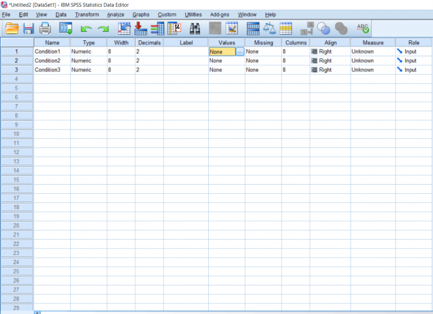
In order to make this easier to understand when I’m actually analyzing the data, I’m going to name each of these numbers using the Values section which is highlighted in the Variable View picture two pictures up. Simply double click it to make the blue button appear and click the blue button for a pop-up to appear.

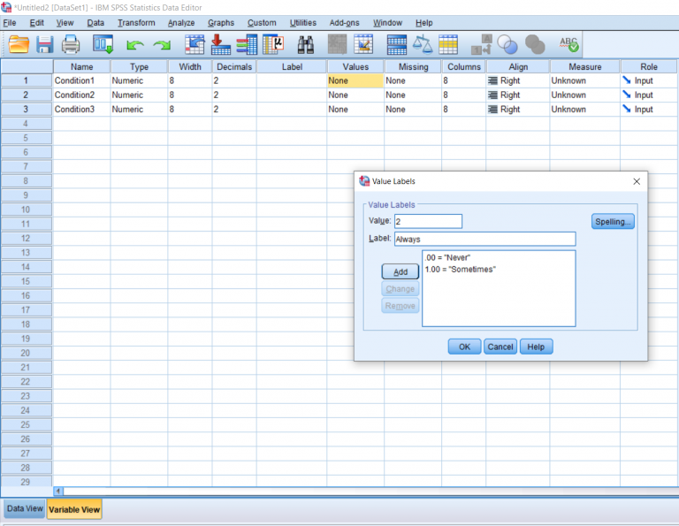
To name a number, simply type the value into the Input box, type the name you would like to give it into the Label box, and click the Add button. When you’re done naming all of your numbers, you can hit the OK button. We won’t be going over what good this does in this post, but it will be important for reading your output data later on, which will be discussed in other posts.

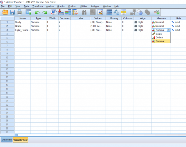
Going back to the Data View, as you can see, changing the names of your data digits does not affect the Data View. I also went ahead and changed the names of the variables in Variable View so that the data have some more context. There are some other things in Variable View which may be important to consider moving forward. Like I said, we’re working with nominal values and SPSS gives us the option of defining them as such for analysis purposes. All you have to do is go back to Variable View, click the button under Measure which corresponds with the variable you would like to change the scale for, and select what you would like from the drop-down menu.

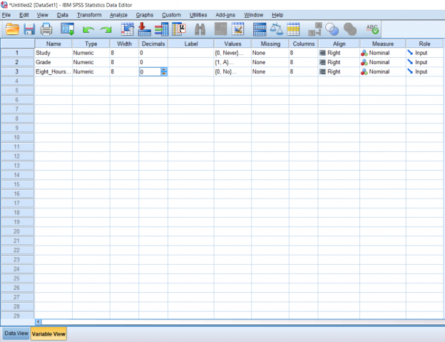
Finally, when I’m working with whole numbers, I find the two decimals at the end of each number to be rather annoying. To get rid of those, just click the box you want to change under Decimals and change the number of decimals you would like to see next to each number in that variable column.

These are all the basics of inputting data. It is possible to copy and paste Excel data into SPSS if you already have a data set ready. Please just keep in mind that unlike working in Excel, variable names cannot simply be put in the first rows of the sheet, they must be logged in Variable View.

This chapter was originally posted to the Math Support Center blog at the University of Baltimore on June 30, 2019.

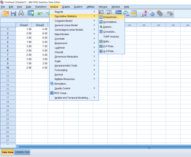
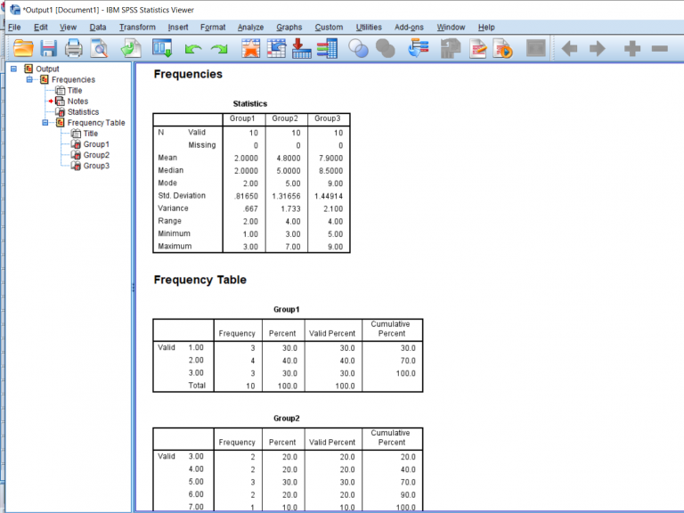
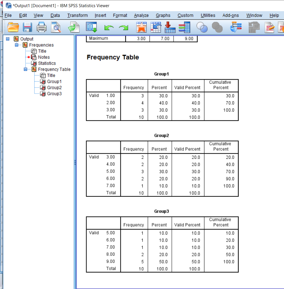
Sometimes you’ll want to get some basic information on the data you have. Running these descriptive statistics is pretty straight forward. First, click the Analyze button, hover over the Descriptive Statistics tab, and then you’ll be able to choose a few different options. I prefer just clicking the frequencies button because it gives you the option to look at frequencies as well as other kinds of descriptives.

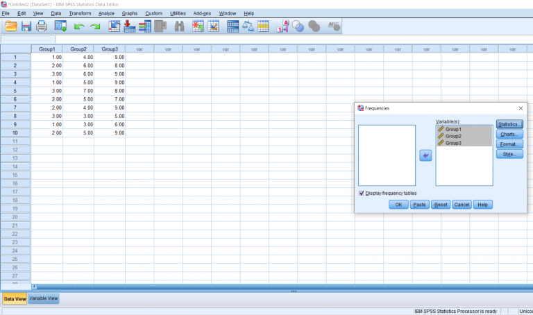
After clicking that, a pop-up will appear. Highlight the groups you would like descriptives and frequencies on and move them over to the right.

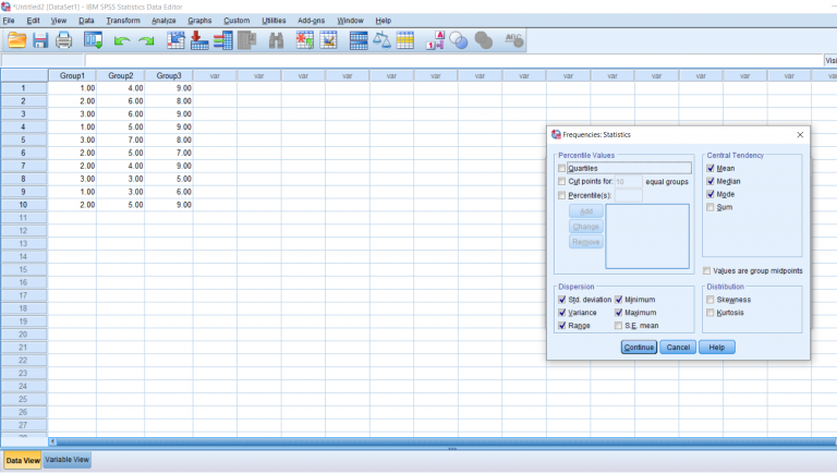
To get the descriptive data we want, click the Statistics button. You can choose from a variety of different descriptives. I like getting all the measures of central tendency and everything related to variability, but as you can see there are other options as well.

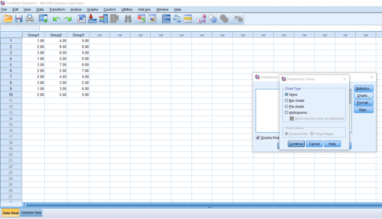
After clicking out of that, you can then have SPSS make you a chart or a graph by clicking the Charts button. I decided not to go ahead with that, but I wanted to point out that option. There are some other buttons to click, but I personally have never needed to mess with those.

Once you finish with the pop-up, the output should appear on a separate window. These are screenshots of what my data looked like. This output is pretty easy to read because it’ll just tell you what you asked to know. Other outputs may be more difficult to read so in future posts I’ll go into detail about what it is you’ll be looking at.

This chapter was originally posted to the Math Support Center blog at the University of Baltimore on July 1, 2019.

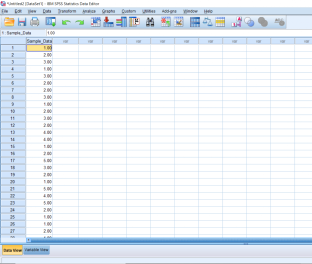
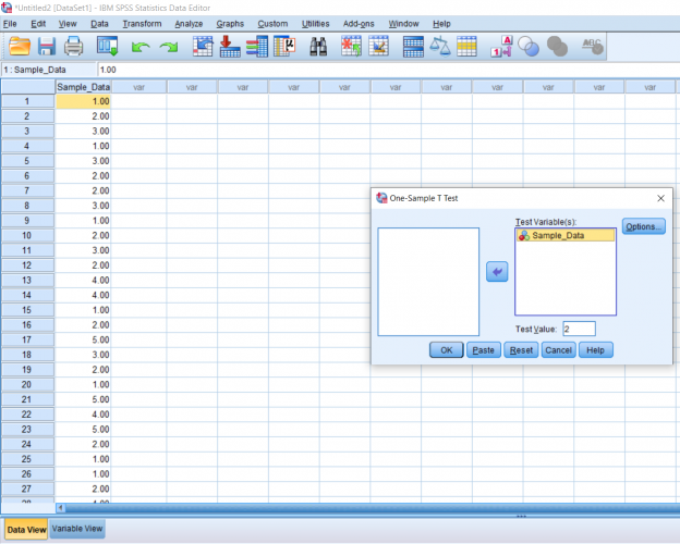
With a one-sample t-test, we only need to worry about working with one sample. When starting, you should already know the population mean you’ll be comparing the sample to. So in this first picture, we have one column of data lined up and ready to go.

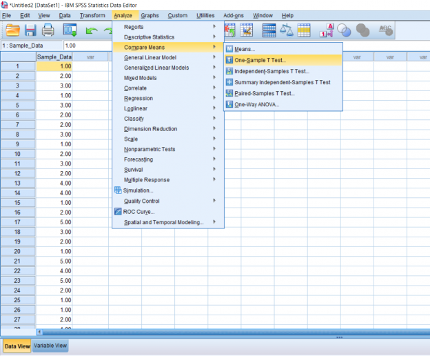
The next step is to click the Analyze button, hover over Compare Means, and click One-Sample T-Test.

A pop-up should appear. Simply move the name of your test variable to the right. In the Test Variable, type in the population mean you would like to compare the sample to.

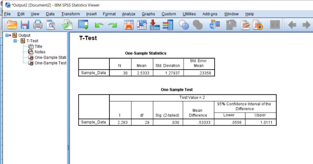
This is what my output ended up looking like. In the first row of boxes, N is the number of data points you have. In the second row of boxes, t is the t-statistic, df is the degrees of freedom, and Sig. is the p-value. The p-value will tell you if the difference is significant. Usually, we look for a p-value less than or equal to .05 before we state that the difference between the means is significant. In this case, the difference is significant.

This chapter was originally posted to the Math Support Center blog at the University of Baltimore on July 1, 2019. 

So far we’ve talked about creating independent variables, but what about levels? This may seem strange at first, but levels of a condition need to be spelled out by numbers. Usually, I just assign condition 1 a 1 and condition 2 a 2. You can see in the picture below how this looks. You can’t see this, but there are 30 individuals in total, half in condition 1, and half in condition 2.

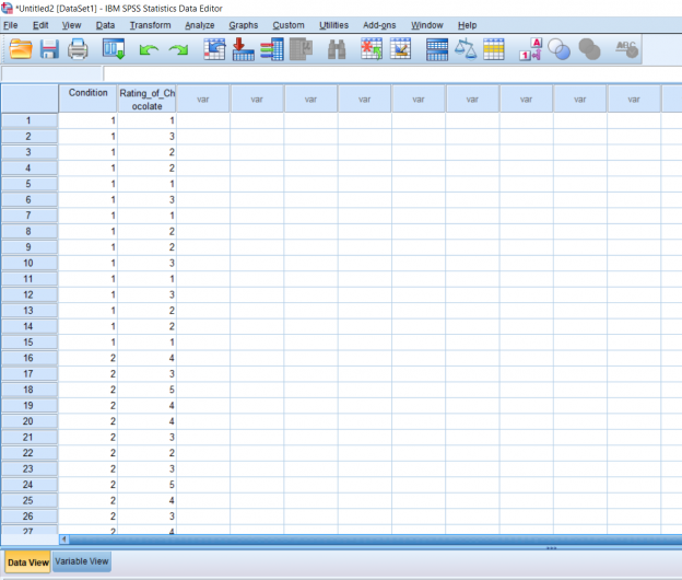
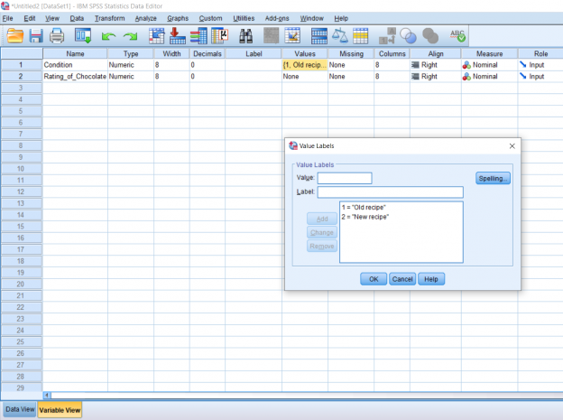
For this tutorial, we’ll pretend that this data has been collected by a struggling baker who wants to try out a new cookie recipe to see if customers would like it better. She asks 15 people to sample her old recipe and 15 people to sample her new recipe and rate how they liked the cookie on a scale of 1-5. To make this easier to read in the output later, I’m going to label the conditions in Variable View.

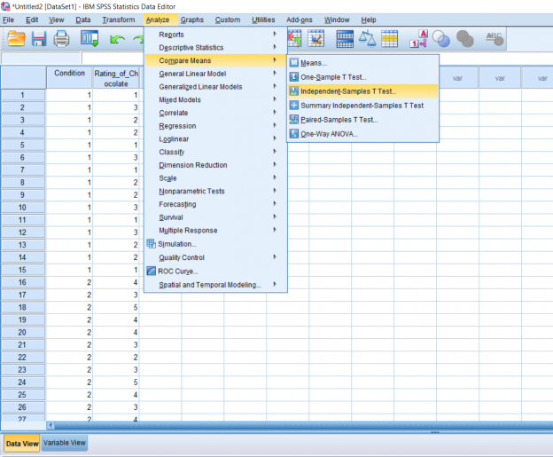
Now it’s time for the actual analysis. Click the Analyze button, hover over Compare Means, and click Independent Samples T-Test.

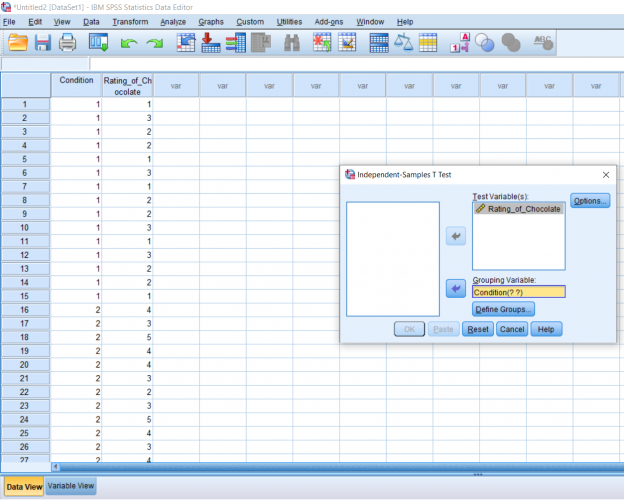
A pop-up will appear. Put your dependent variable in the Testing Variable box and your conditions in the Grouping Variable box. Then, click the Define Groups button.

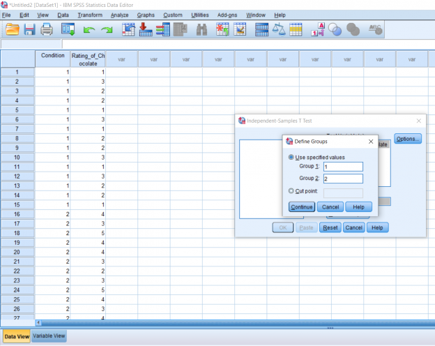
Another pop-up will appear. Simply fill in each box with the number that corresponds to your groups (again, in my case it’s just 1 and 2).

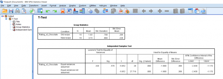
Your output will look something like this. The first row of boxes will simply give you descriptives about your data. The second box get’s a little tricker. The boxes under Levene’s Test for Equality of Variances simply allows the user to see if the two samples have equal variances. In this case, we want the p-value to be less than .05 because we don’t want any differences in the variances. It looks like we’re in the clear for this data set. The next few boxes give us the t-statistic, the degrees of freedom, and the p-value. It looks like our conditions are significantly different. Remember to report a .000 p-value as p<0.01, because there is no such thing as a p-value of 0. So we know that there’s a difference, but which cookie got the higher score overall? Simply look at the means. The new recipe has a higher mean rating than the old recipe.

This chapter was originally posted to the Math Support Center blog  at the University of Baltimore on July 1, 2019. 

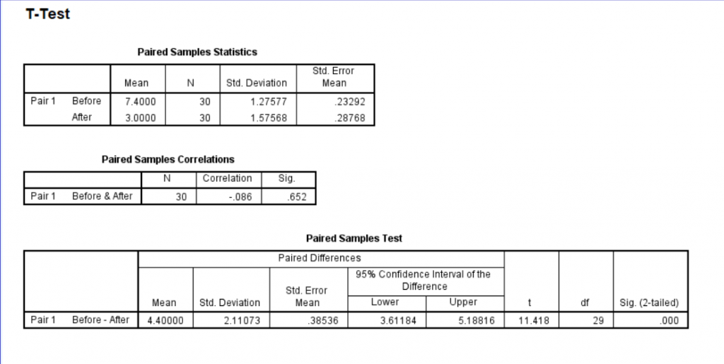
In this section, we’ll be talking about how to properly conduct a repeated measures t-test on SPSS. Before, when we were working on independent t-tests, we needed to create a list of numbers which represented group categories so that the corresponding continuous data was grouped properly. In this kind of t-test though, each “Variable” actually becomes a level. In this case of this example, we’re looking at the data from a before and after. The “Before” consists of the number of alcoholic drinks 30 college students are consuming a week. The “After” consists of the number of alcoholic drinks the same college students were drinking after having taken a Wellness class which focused on the effects of drug and alcohol on the mind and body. If you’re confused as to how this differs from an independent samples t-test, I suggest looking at the Independent Samples t-test and Repeated Measures t-test chapters.

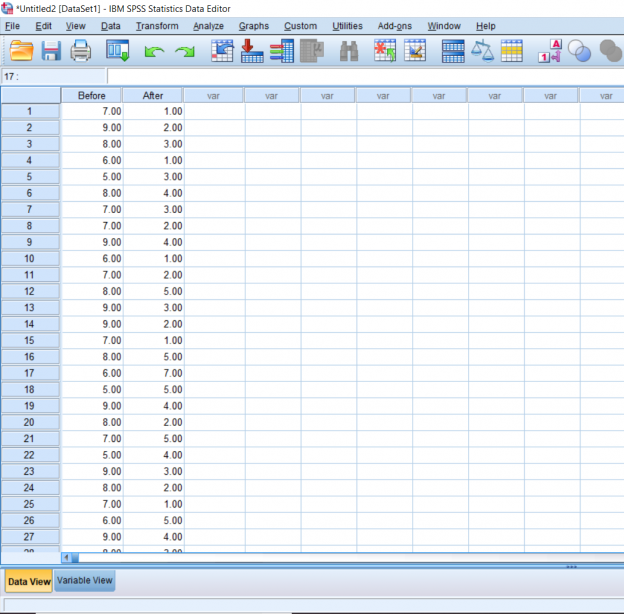
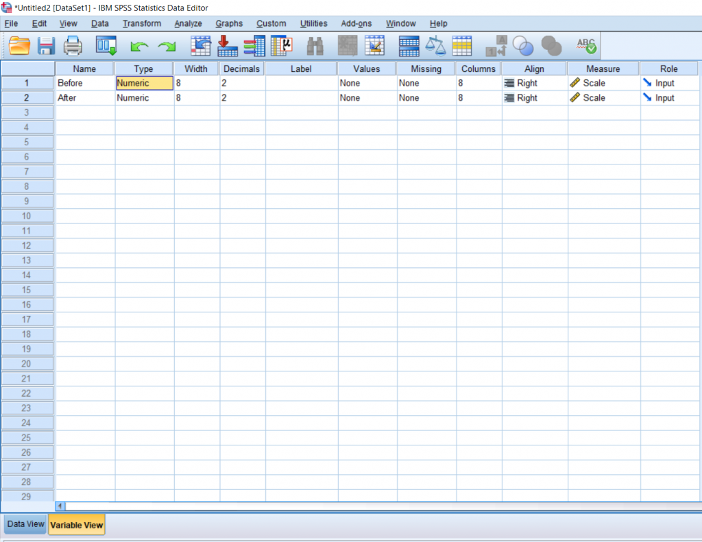
Just for reference, I have already labeled my columns Before and After in the Variable View section.

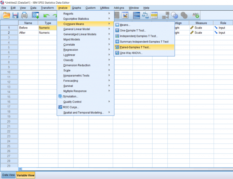
To conduct the test, click the Analyze button, hover over Compare Means, and click Paired Samples t-test.

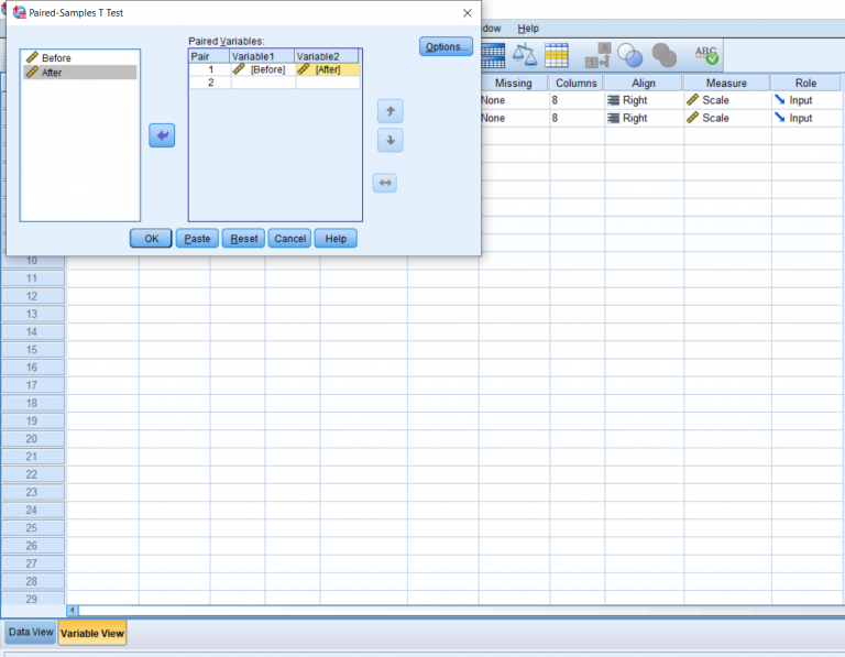
Simply drag your before and after into the correct slots. These are usually done in chronological order from left to right.

Finally, you’ll get your output. Based on this particular test, we can see that we got a t score of 11.4, which is already a pretty good indicator that the results will be significant. Typically, anything above a 3 or 4 will be significant. Just to be sure, let’s look at our p value. It’s less than 0.05, which is our typical alpha level, which means that there was a significant difference between the before and after. To see in which direction there is a difference, we go up to the means. Which one is smaller or bigger than the other? We can see that the mean drinks before the intervention was higher on average than after the intervention. In this case, we would say participants drank significantly fewer drinks per week after the intervention than before the intervention.

This chapter was originally posted to the Math Support Center blog at the University of Baltimore on July 16, 2019.

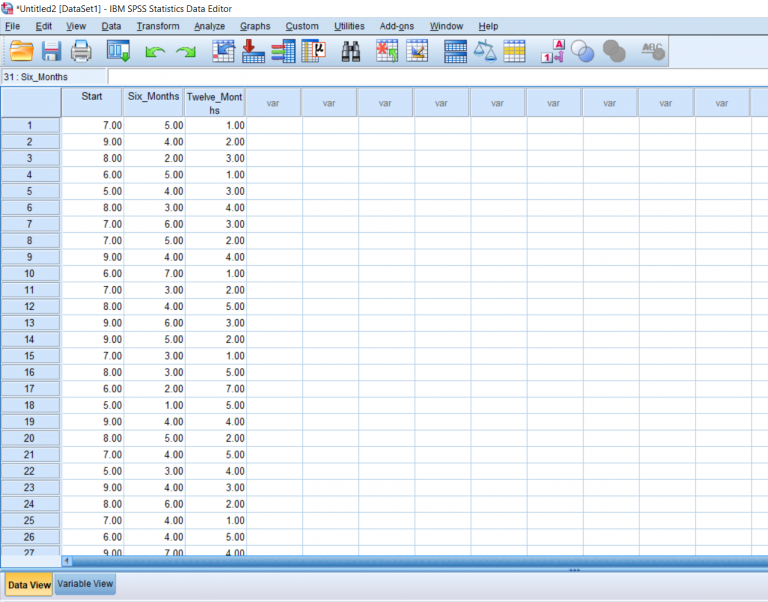
This post will be about finding a difference in means when it comes to repeated measures in research designs with a factor with more than 2 levels. Just like with the Repeated Measures t-test, we’ll be lining our levels up in columns. For this example, we’ll pretend that we’ve collected data on self-reported depression. Participants were asked to rate on a scale from 1-9 how severe they felt their depression is. They were then given medication to take which is known to reduce depressive symptoms. Participants were asked again after 6 months how high they rated their depression. They were asked one last time at the end of 12 months.

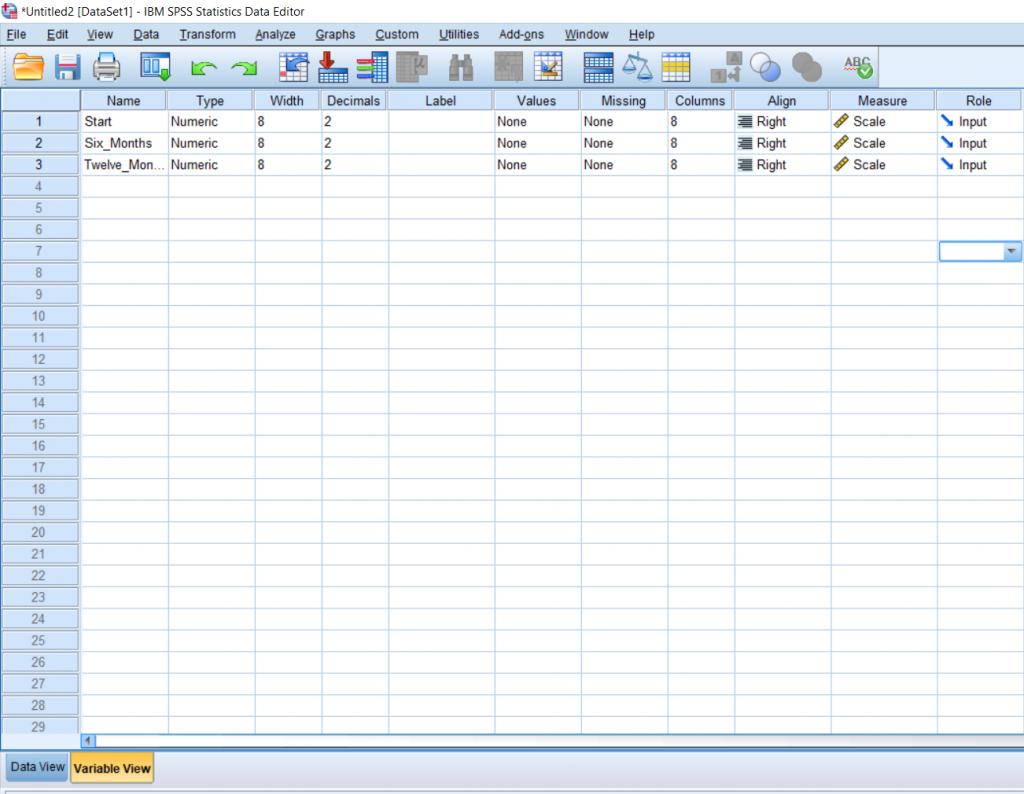
I went ahead and named the levels in the Variable view.

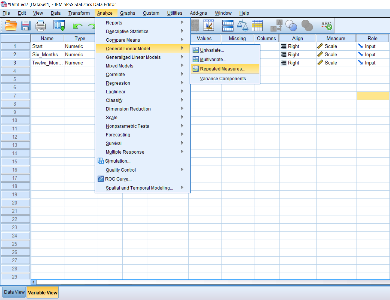
To run the actual test, simply go up to Analyze, scroll over General Linear Model, and click Repeated Measures.

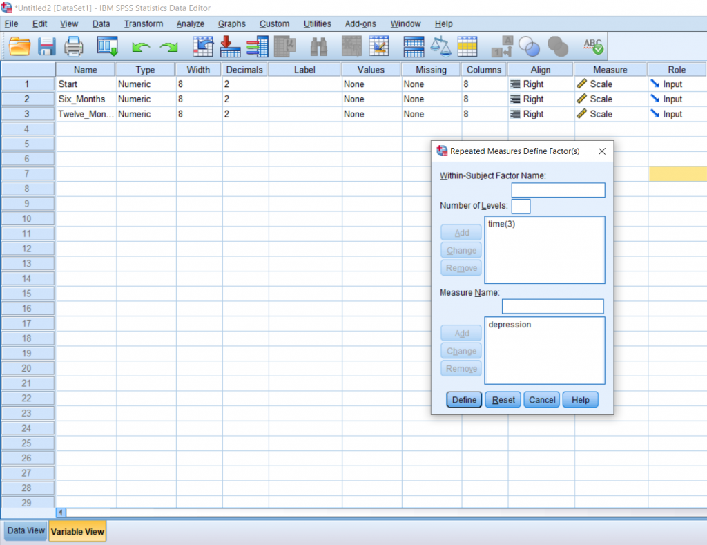
A pop-up will appear. In the first box, create the name of your factor. In this case, I’ve named it time, because we’re doing comparisons across time. In the second box, I typed in 3 because we have 3 levels and then I pressed Add. In the third box, I named our dependent variable and clicked Add. Next, we need to Define our factors.

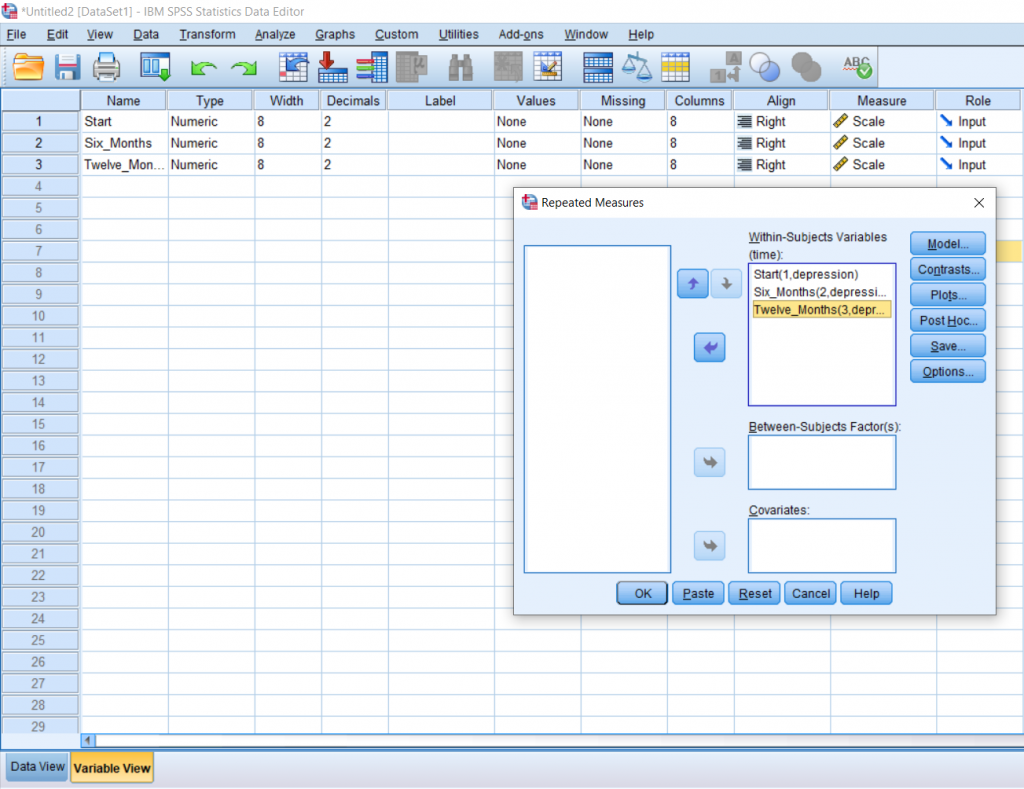
Another pop up will appear. Move the levels over into the top, right box. I prefer doing this in chronological order from top to bottom. Then, click Options.

I would recommend getting means for everything, so move OVERALL and time over to the box on the right. I also recommend clicking the Descriptive Statistics and Estimate of Effect Size boxes. Finally, click the Compare Means checkbox; it’s located under the big, white box on the right. Click all the Continues and OK’s that follow.

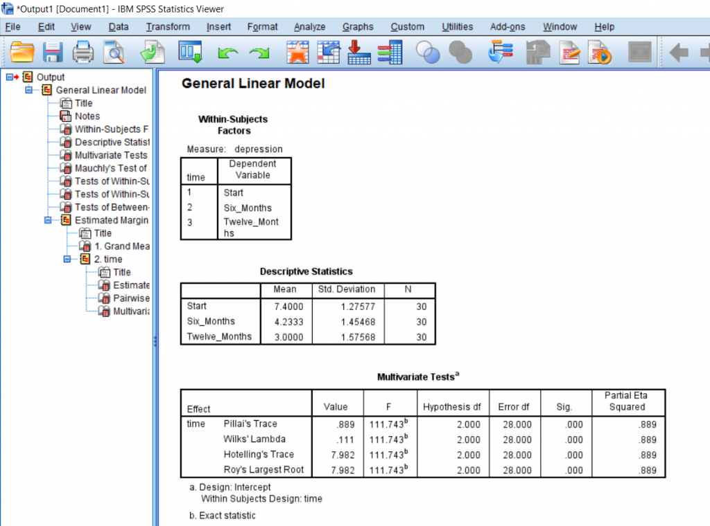
We can see from the means that the average for Start is greater than at 6 months is greater than at 12 months. This is important to know, but this does not prove significance.

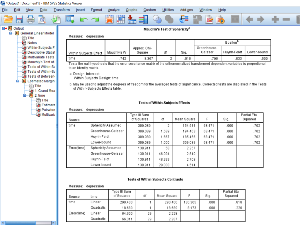
Go to the Tests of Within-Subjects Effects box and find “time” on the left, scroll over to Greenhouse-Geisser, and then scroll all the way to F and significance. We have a huge F score of 68.5 and a significance which is less than 0.05 and so we can say that somewhere there is a significant difference in the groups. If you need to report the effect size, you can find it under Partial Eta Squared.

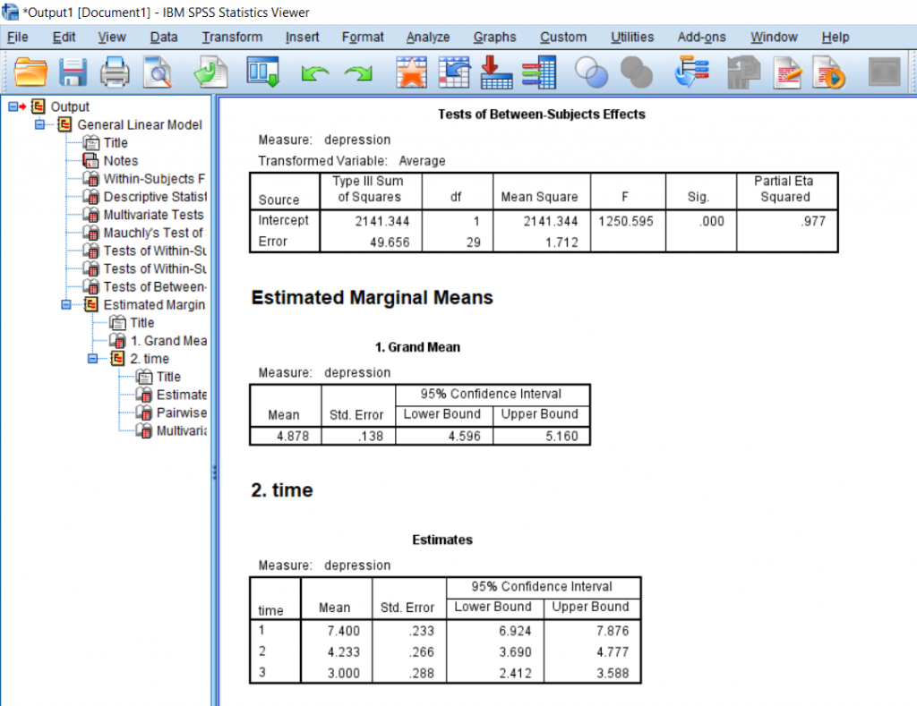
This last box shows us the post-hoc under Pairwise Comparison. As you can see, all the comparisons are significantly different with a significance less than 0.05. This means that we can say that there was a significant difference in times since treatment began with participants expressing the most depression before the treatment started, less depression 6 months after the treatment started, and the least depression after 12 months of treatment.

This chapter was originally posted to the Math Support Center blog at the University of Baltimore on July 16, 2019.

Just like an independent samples t-test, an Independent measures one-way ANOVA uses independent subjects for each level/condition within an independent variable. In this example, we’re growing plants. In Variable View, I’ve made the independent variable Condition (in this case the amount of water I’ll be giving to the plants) and the dependent variable Height.

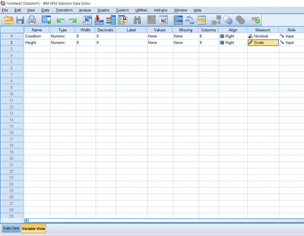
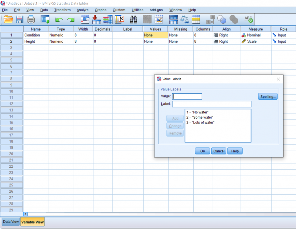
Next, it’s important to label the levels of your independent variable, so I clicked the cell under Values and assigned the numbers 1, 2, and 3 a condition: no water, some water, and a lot of water.

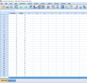
Then, I just put my data in Data View, with the Condition column full of the numbers representing the different conditions and the Height column full of the measured heights of each plant.

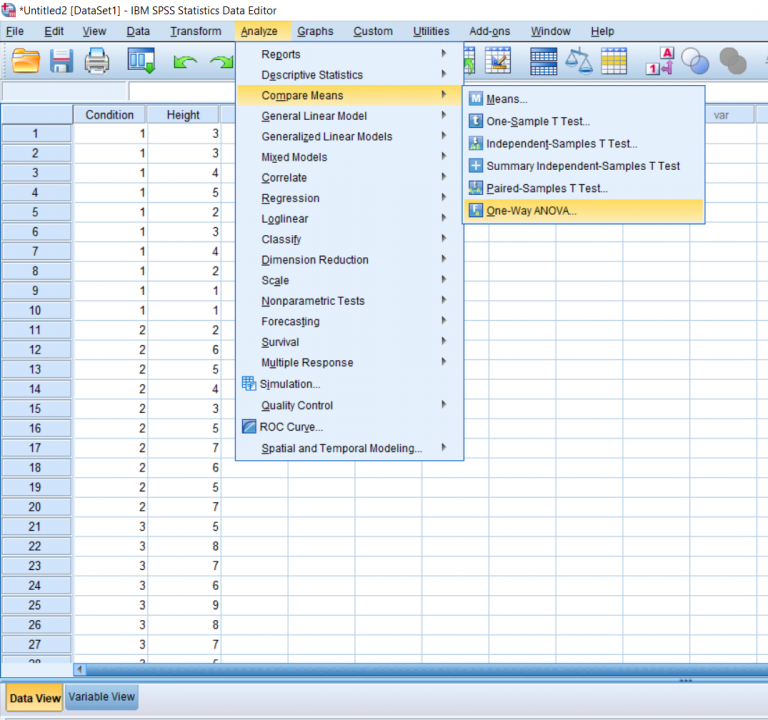
To conduct the test, click Analyze at the top, hover over Compare means, and then click One-Way ANOVA.

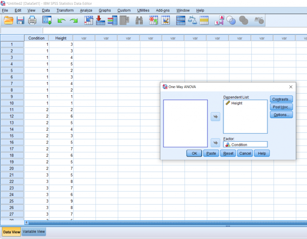
You’ll be greeted with a pop-up asking you to arrange the variables you would like to test. The dependent variable goes in the top box and the independent variable goes in the bottom box. Then, click the Post Hoc box.

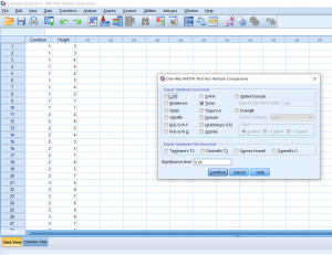
You will be greeted by another pop-up. Here you can click the kind of post hoc test you would like to run. Tukey seems to be pretty popular, so that’s the one I chose. Then, click Continue.

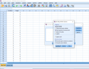
Once back to the main pop-up, then click Options. Here you’ll be able to add in descriptive statistics (like mean, SD, etc.) and a Homogeneity of Variance test, which may be important to report depending on what your professor is asking for. Then, click continue and finally OK.

Your output will look something like this. First is always the descriptives. The next box is the results of the test of homogeneity of variances. Remember, this is the one that we don’t want to be significant; we want there to be no difference between the groups. Looking under Sig, we can see that our p-value is greater than 0.05 so we’re in the clear! The third box shows us the result of our analysis overall. Here, our F-value is 21.4 and we have a p-value of less than 0.01, which means that there is definitely a difference somewhere between these three conditions.

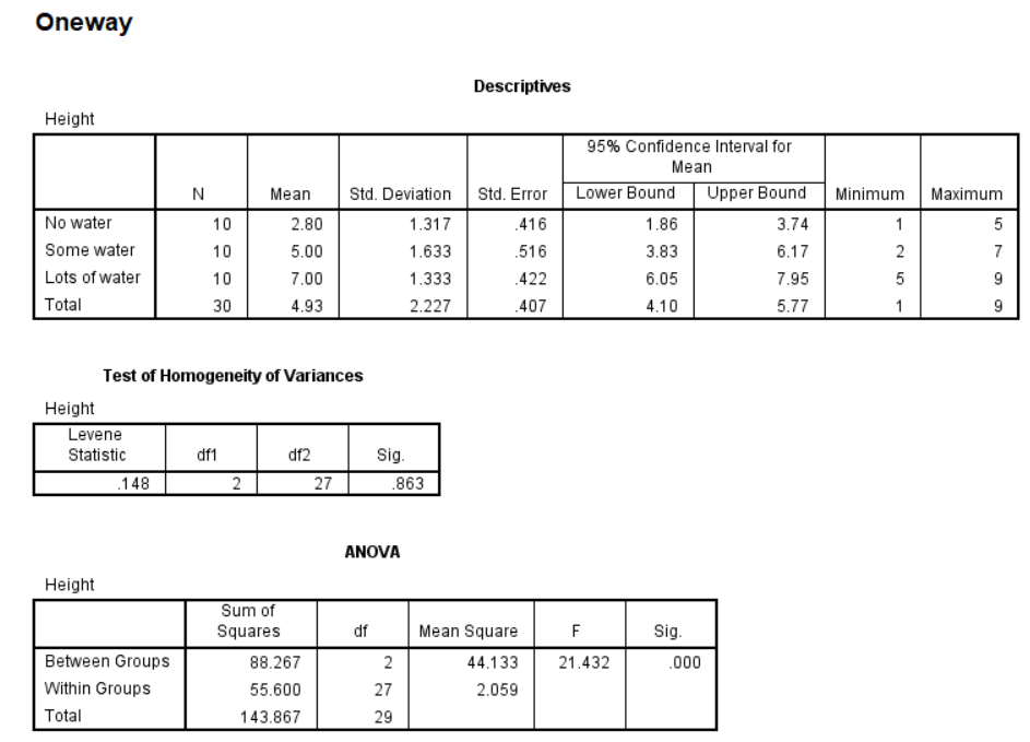
Moving on the Post Hoc, each box compares one group with the other group. So as well can see, no water and some water are significantly different, and no water and lots of water are significantly different (remember that stars indicate significance). We’ve compared conditions 1 and 2 and conditions 1 and 3, but we still need to compare 2 and 3, so we move down to the next box and see that some water and lots of water are also significantly different. Make sure to report all of these differences. To know which groups are significantly less than or greater than others, refer to the descriptive statistics at the top (specifically the means).

This chapter was originally posted to the Math Support Center blog at the University of Baltimore on September 10, 2019. 

A regression can be seen as a kind of extension of a correlation. When doing a regression, you find a lot of the same outputs, like Pearson’s r and r-squared. The difference is that the point of a regression is to also construct a model (usually linear) that will help us predict values using a line of best fit. In the case of this example, we will be looking at average hours of sleep students get and comparing it to their GPA. A regression will also give us a model (y=mx+b) that would allow us to predict the GPA of a hypothetical student if we knew the average amount of sleep they get a night.

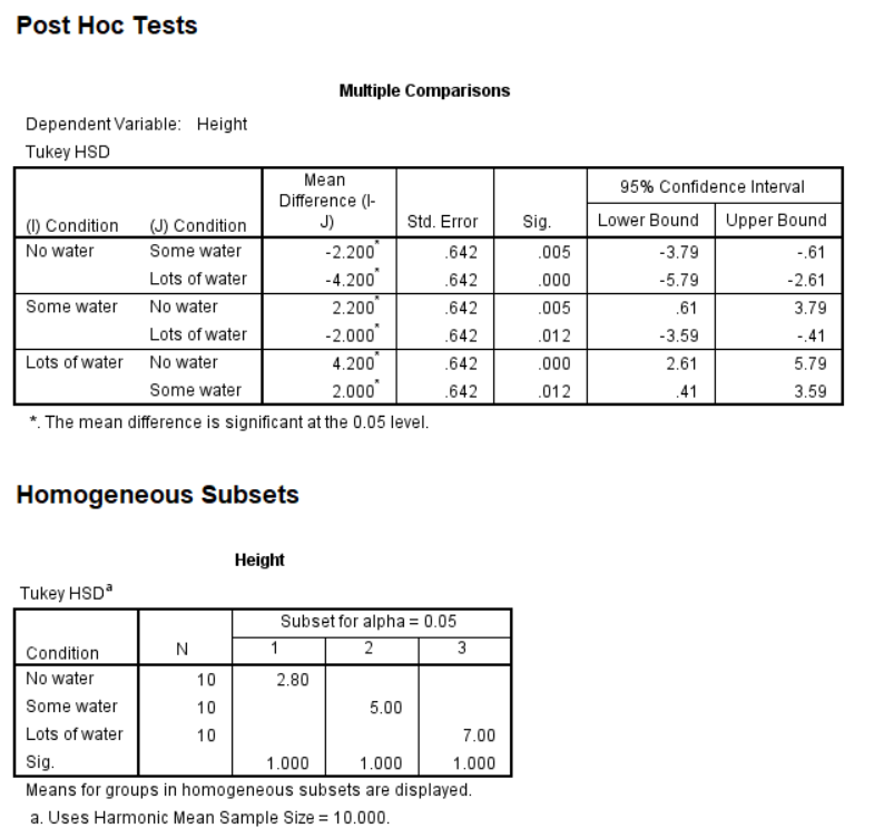
First, we need to create our variables in Variable View.

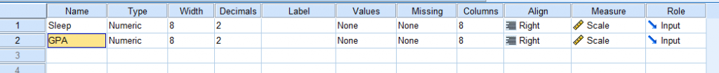
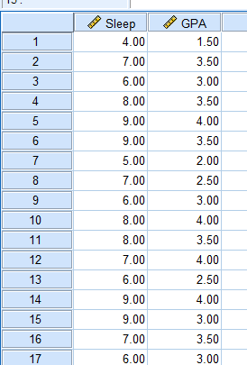
Then, we need to input our data into Data View. You can’t see it in this photo, but I have 25 participants total.

To start our regression, we need to go to Analyze > Regression > Linear.

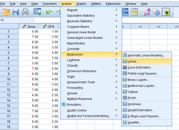
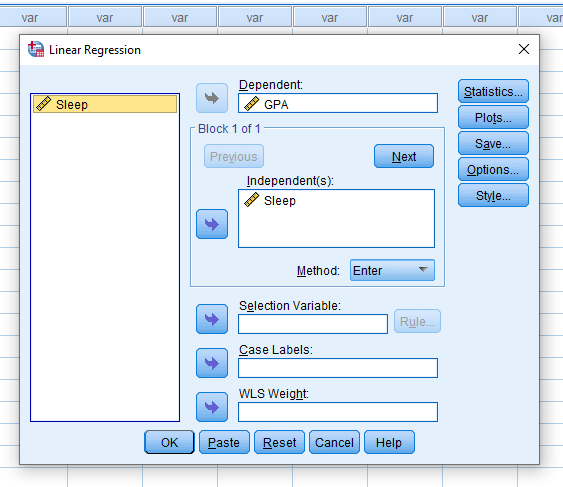
Once we click that, this pop-up will appear. Make sure to make your predictor the independent variable and the predicted variable the dependent variable.

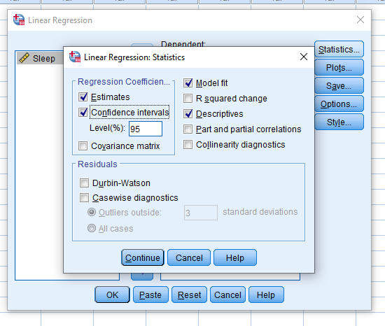
It may be important for you to then click the Statistics button and make sure to check what you need to include in your report. Descriptives and Confidence Intervals never hurt.

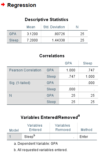
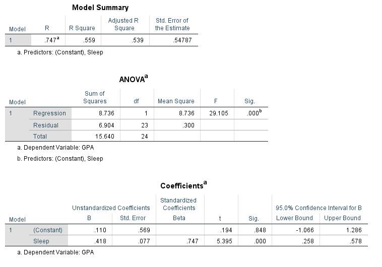
Your output will look something like the following two pictures. Descriptives are at the top, so this will help you report your means and standard deviations if you need to. Next are your correlation matrices. In my case, it looks like Sleep and GPA have a somewhat strong positive correlation and it appears to be significant with a p- value of less than .001. Ignoring the variables entered/removed section, the model summary shows us once again our r value and it also gives us an r-squared value. The ANOVA table gives us an F value and significance if we choose to report that. Finally (and the part we’ve been waiting for) is the model. This part is like in Algebra when you needed to learn about linear functions. We’re constructing a line using y=mx+b where the m is the slope and the b is the y-intercept. For this example, the model we’re working with is y=0.11x+.418 and I found these numbers from the coefficients table.

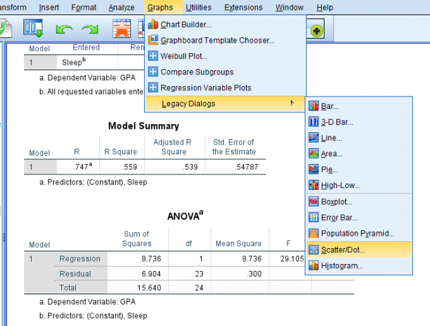
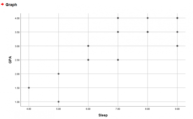
Now let’s say you need a graph of this. Go to Graphs > Legacy Dialogues > Scatter Plot.

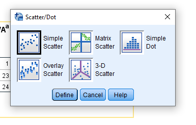
This pop-up should appear. Just click Simple Scatter.

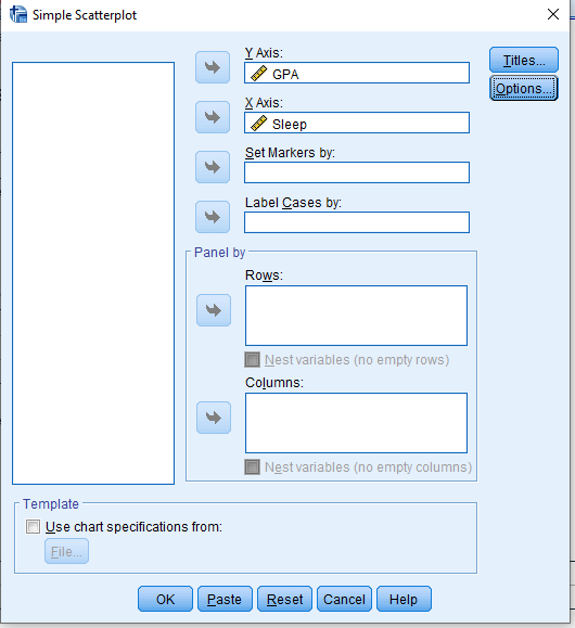
Another pop-up should appear. Make sure your predictor is on the x-axis and the predicted variable is in the y-axis.

You should end up with this basic scatterplot of your points.

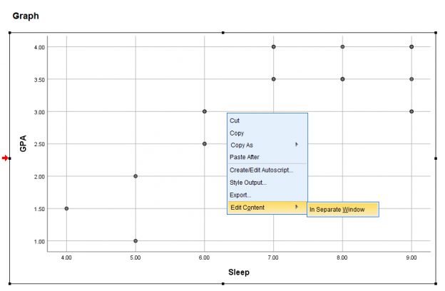
To get the line of best fit, right-click the graph > Edit Content > In Separate Window.

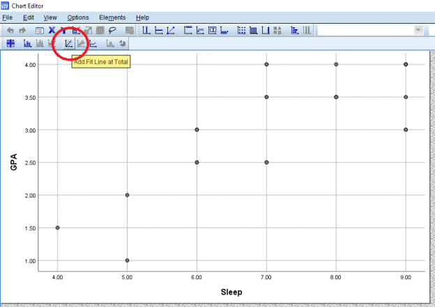
A new editing pop-up will appear. Click the linear equation button at the bottom of the bar. It will say Add Fit Line at Total when you hover over it.

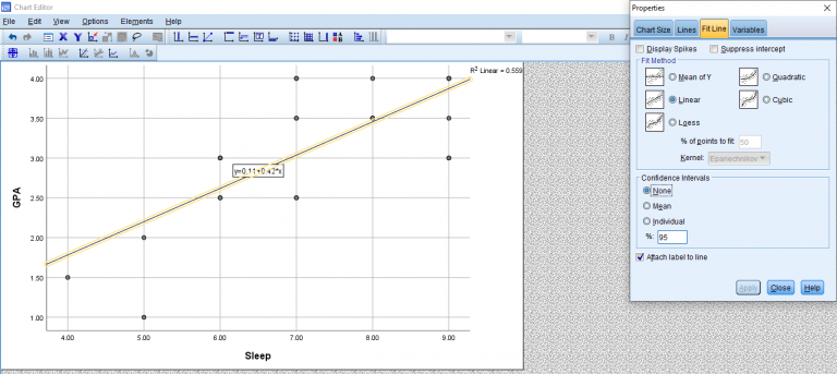
Once that’s done, your graph should look something like this. If you exit out of the pop-up to go back to the output, the output graph should represent the changes you made in the editor pop-up.

This chapter was originally posted to the Math Support Center blog at the University of Baltimore on February 11, 2020.

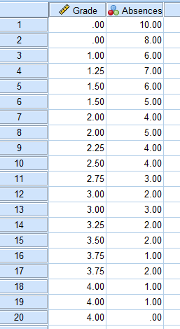
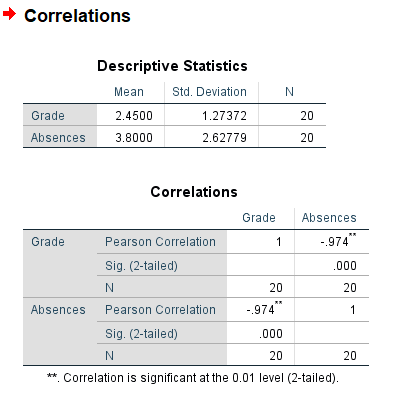
A correlation requires at least 2 continuous variables. We need to first define our variables in Variable View. In this case, we’re looking at how number of absences relates to grade point average.

Next, we type in our data points in Data View.

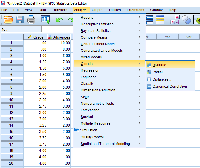
To run the analysis, go to Analyze > Correlate > Bivariate.

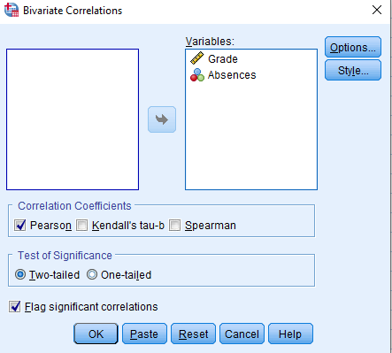
A pop-up should appear. Put both of your variables in the Variables column.

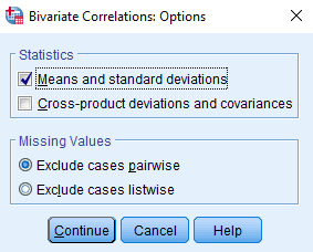
Then, go to options and click means and standard deviations if that is something you need to report.

Your output should look something like this. The correlations matrix looks a little redundant, but what’s important here is the Pearson Correlation value and the significance. You should have everything you need here to report a correlation. For information about how to do a scatter plot, please visit the SPSS Regression chapter.

This chapter was originally posted to the Math Support Center blog at the University of Baltimore on February 13, 2020.

Whether this is your first statistics class or whether you’re just in need of a refresher, there are a few basic statistical principles which are necessary for one to understand before moving forward.

Understanding Populations and Samples

Populations are the groups of people that we are interested in studying. This can be the entirety of people with depression, an entire town, or dog-owners. Populations can vary in size but are typically very large. They are almost always impossible to study in their entirety. Therefore, we select samples from a population. Although they’re never as diverse as the population, they are generally representative. However, they provide limited information and introduce sampling error.

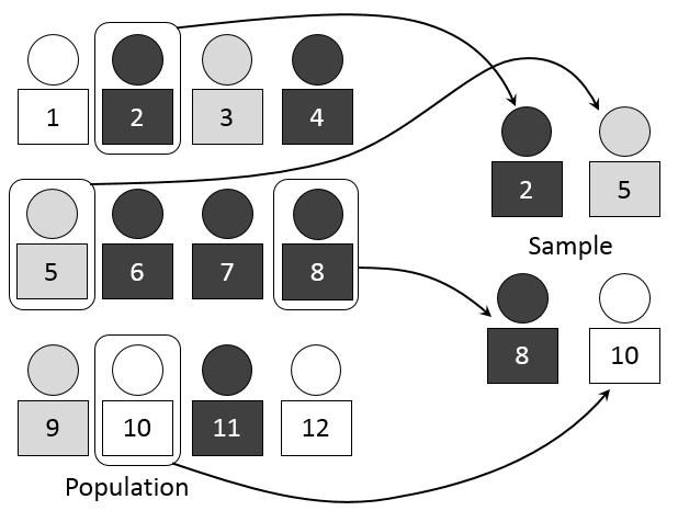
Samples are a subset of the population which as been selected by various means. A sample is representative when it accounts for the variability and diversity of the population. For example, a representative sample of “individuals who attend the University of Baltimore” would include a diversity of age groups, race, educational background, students from different programs, faculty from multiple departments, staff, etc., in their appropriate percentages in the population. A non-representative sample in that case would not account for the various differences that exist among the individuals in a population, or would over-represent/under-represent a specific group. The figure below illustrates a hypothetical population, two examples of non-representative samples, and one representative sample of that population.

Created by Dan Kernler and shared under a CC BY-SA 4.0 License

Why do we care about these distinctions? What we really care about is getting an answer that most closely represents a population. A non-representative sample introduces bias and error, and precludes researchers from making sound interpretations. But since we can’t study entire populations, we want to take samples and study them as best as we can to generalize the results to the population. Samples are not going to be exactly representative of a population so it’s best to know the distinction.

Why can’t researchers study entire populations? As we mentioned before, populations are usually extremely large, and it would require a lot of time and resources (e.g. financial resources) to study it in its entirety. Furthermore, in a hypothetical world where a researcher possesses the resources necessary to do so, they will not be able to include every single person from the population in their research study.

Parameters vs Statistics and Sampling Error

A parameter is a value that describes a population, while a statistic is a value that describes a sample. A good way to remember it is: Parameter – Population, Statistic – Sample. If the sample was a good enough sample (completely random and preferably large), then these values should be very similar. Sampling error is the discrepancy that exists between a sample statistic and the corresponding population parameter. Every sample will have sampling error simply because a sample cannot possibly be as diverse as a whole population, but there are measures of preventing a larger one.

How do these things relate to one another? These things all relate to each other because we select participants from a population which become a sample, on which we run tests and analysis, and then we can determine if the results are then generalizable to the general population we’re studying.

Sampling Methods

There are a number of ways to collect sample data. There are pros and cons to each, but simple random sampling reduces sampling error the most.

• Simple Random Sampling:
  • Everyone has an equal chance of being selected.
  • The selection method is completely random.
  • One individual’s selection does not impact the likelihood that someone else is subsequently selected.
• Systematic Sampling:
  • In a lost of all the individual, every nth individual is picked.
• Convenience Sample:
  • Using the first individuals a surveyor comes across for the sample.
  • Least likely to get a representative sample.
• Cluster Sampling:
  • Dividing the population into groups (usually geographically).
  • The clusters themselves are randomly selected while the people in them are not.
• Stratified Sampling:
  • Divides the population into groups based on characteristics.
  • A sample is taken from each of these groups so that characteristics that are important are accounted for.

Variable Types and Individuals

A variable is a characteristic or condition that changes or has different values for individuals. In other words, it’s something that can be manipulated, categorized, or measured. An independent variable is a variable that is manipulated or decided on by the researcher. A dependent variable is a variable which is not to be manipulated, but instead observed. For example, if one is trying to see whether plants grow faster depending on the type of fertilizer is used, then the independent variable is the type of fertilizer and the dependent variable is the growth of the plant.

A categorical variable is a variable which is measured by its name or category. This could be color (red, green, blue, etc.), gender (man, woman, nonbinary, etc.), or in the case of our coffee example, whether the coffee is meant to be served hot or cold. Although we might assign each of these categories a number in SPSS or excel, these numbers have no quantitative value and are just replacements for the names. Here is a Khan Academy video which may be helpful to you in understanding this concept:

A YouTube element has been excluded from this version of the text. You can view it online here: https://ubalt.pressbooks.pub/mathstatsguides/?p=56

An individual is an object or person that is described by a set of data. So if we were measuring the height and weight of 15 participants, each of those participants would be an individual in the study. If we were looking at the different coffees on a menu and we gathered data on whether each drink is hot or cold, how many calories is in each drink, how much sugar is in each drink, and how much caffeine is in each drink, then each of the different kinds of coffee would be considered individuals in this study.

Types of Statistics & Types of Studies

Descriptive statistics are used to summarize, organize, and simplify data (basically it lets us turn data sets into something legible). Inferential statistics are techniques that allow us to make generalizations about the population from a sample (so this is actually comparing groups to see if there are statistical differences between them or comparing variables to see if there are relationships between them). There are two types of data structures that make use of these kinds of statistics.

Data Structure I: Measuring two variables for each individual

Correlational method: Measuring two variables for each individual in order to determine if there is a significant relationship between the two. A limitation of this method is that it can show a relationship, but not an explanation for the relationship. A correlation does not necessarily mean a causation and is never enough to draw such an inference.

Data Structure II: Comparing two or more groups of scores

Experimental Method: The goal is to demonstrate a cause and effect relationship between two variables. The experiment attempts to show that changing the value of one variable causes changes to occur in the second variable. This requires:

• Manipulation: The researcher manipulates one variable by changing its value from one level to another. A second variable is observed to determine whether the manipulation causes changes to occur
• Control: The researcher must exercise control over the research situation to ensure that other, extraneous variables do not influence the relationship being examined. These variables that need to be controlled can be participant variables (characteristics such as age, gender, and intelligence that vary from one individual to the other) or environmental variables (lighting, time of day, weather, etc.). Researchers should control for as many variables as they can, and so spend a lot of time designing an experiment about what variables are important to control for and how to go about doing that.

Non-experimental Method (Nonequivalent groups and pre-post studies): This is when the experimenter is unable to fully manipulate the independent variable. For example, when gender is studied, one can’t assign participants to be a random gender. Researchers also have no control over time, and so pre-post tests are also not true experiments. What is meant by this is that a variable is measured twice (pre and post), and researchers can’t control which they measure first – it must be the pre.

Constructs

Constructs are internal attributes or characteristics that can’t be directly observed but are useful for describing and explaining behavior. The construct is a proposed attribute of a person that often cannot be measured directly, but can be assessed using a number of indicators or manifest variables (for example, depression). We tend to use an operational definition for constructs, which describe a set of operations for measuring the construct and defines a construct in terms of the resulting measurement. Here is a helpful YouTube video for explaining this concept:

A YouTube element has been excluded from this version of the text. You can view it online here: https://ubalt.pressbooks.pub/mathstatsguides/?p=56

Scale Types

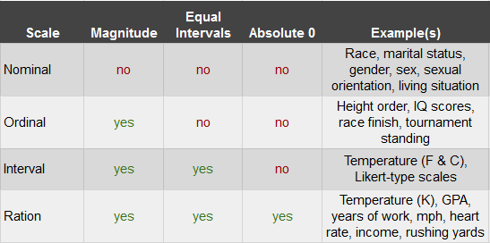
A scale is a way in which to categorize and/or quantify variables. Each type of scale may have a combination of magnitude, equal intervals, absolute 0, or none. Magnitude means that the scale specifies if each marker has relative value to the other markers. Equal intervals means that a one point difference carries the same weight throughout the scale and that there is a linear relationship among the variables. Absolute 0 just means that the 0 on the scale means the complete absence of that thing. The different types of scales are as follows:

• Nominal: Set of categories; no quantitative distinction (Ravens, Steelers, etc.)
• Ordinal: Categories in an ordered sequence ( 1st place vs. 4th place. We don’t know the differences between each race time, only that this is the order that they came in.)
• Interval: Ordered categories with equal intervals. Arbitrary zero point (ex. Celsius, 0 could have been placed anywhere but we decided to place it at the freezing point of water)
• Ratio: Ordered categories with equal intervals. Absolute zero point. (ex. Height or weight)

This chapter was originally posted to the Math Support Center blog at the University of Baltimore on June 4, 2019.

In statistics, a lot of tests are run using many different points of data and it’s important to understand how those data are spread out and what their individual values are in comparison with other data points. A frequency distribution is just that–an outline of what the data look like as a unit. A frequency table is one way to go about this. It’s an organized tabulation showing the number of individuals located in each category on the scale of measurement. When used in a table, you are given each score from highest to lowest (X) and next to it the number of times that score appears in the data (f). A table in which one is able to read the scores that appear in a data set and how often those particular scores appear in the data set. Here’s a Khan Academy video we found to be helpful in explaining this concept:

A YouTube element has been excluded from this version of the text. You can view it online here: https://ubalt.pressbooks.pub/mathstatsguides/?p=66

Organizing Data into a Frequency Distribution

1. Find the range
2. Order the table from highest score to lowest score, not skipping scores that might not have shown up in the data set
3. In the next column, document how many times this score shows up in the data set

Organizing data into a group frequency table

1. The grouped frequency table should have about 10 intervals. A good strategy is to come up with some widths according to Guideline 2 and divide the total range of numbers by that width to see if there are close to 10 intervals.
2. The width of the interval should be a relatively simple number (like 2, 5, or 10)
3. The bottom score in each class interval should be a multiple of the width (0-9, 10-19, 20-19, etc.)
4. All intervals should be the same width.

Proportions and Percentages

Proportions measure the fraction of the total group that is associated with each score (they’re called relative frequencies because they describe the frequency in relation to the total number of scores). For example, if I have 10 pieces of fruit and 3 of them are oranges, 3/10 is the proportion of oranges. On the other hand, percentages express relative frequency out of 100, but essentially report the same values. Keeping in line with our fruit example, 30% of my fruit is oranges. Here’s a YouTube video which might be helpful:

A YouTube element has been excluded from this version of the text. You can view it online here: https://ubalt.pressbooks.pub/mathstatsguides/?p=66

Real Limits

Real limits are continuous variables require a calculation of a real limit. They can be calculated by taking the apparent limit and subtracting and then separately adding half the value of the smallest digit available or presented. For example, I have a value of 50 and I want the real limits. To make it easier to see, I make the number 50.0. The smallest digit shown is the 1 digit, so I subtract half of one (49.5) and add half of one (50.5). Sometimes one isn’t the smallest digit. If I have a value of 34.5, I add another digit to the end to make 34.50, and the smallest value is the 0.5, so we divide by 2 to get 0.25. So the limits are 34.75 and 34.25. Finally, sometimes the smallest value of measurement is given. If the smallest unit a scale can measure is 0.2 pounds, and you have a value of 80 pounds, you add and subtract half of 0.2 pounds and get 80.1 and 79.9. This can be a difficult concept two grasp, so here are two YouTube videos we found helpful.

Frequency Distribution Graphs

A frequency distribution is often best grasped conceptually though the use of graphs. These graphs are like the tables in that they represent the same data, but graphs show it in a different way. This can be done with bar graphs (discrete), histograms (continuous), or polygons (continuous). Here are two Khan Academy videos we found helpful.

These graphs can come in a multitude of shapes, but here are just a few important descriptive words generally used in statistics:

• Symmetrical: When the shape of the distribution is, at least for the most part, mirrored on both sides if you were to view the mean as the flipping point.
• Asymmetrical: When the shape of the distribution is not mirrored on both sides for whatever reason (usually because of skew).
• Positively Skewed: This is when there is what looks like a tail of data trailing off to the right. I like to remember this is as the P in Positive having fallen on its back.
• Negatively Skewed: This is when there is what looks like a tail of data trailing off to the left.
• Unimodal: This literally means having a buildup of data around what looks to be one number, so one mode. Your typical bell curve is unimodal.
• Bimodal: This is when there is data clustering around two different numbers or spots on the distribution, so having two modes. This can often look like camel humps.
• Multimodal: When a distribution has two or more “humps” in the graph.

Here’s a video which may be helpful in teaching you how to interpret data presented in a table and organizing data into a frequency distribution graph.

A YouTube element has been excluded from this version of the text. You can view it online here: https://ubalt.pressbooks.pub/mathstatsguides/?p=66

This chapter was originally posted to the Math Support Center blog at the University of Baltimore on on June 4, 2019. 

Central tendency is a statistical measure; a single score to define the center of a distribution. It is also used to find the single score that is most typical or best represents the entire group. No single measure is always best for both purposes. There are three main types:

• Mean: sum of all scores divided by the number of scores in the data, also referred to as the average.
• Median: the midpoint of the scores in a distribution when they are listen in order from smallest to largest. It divides the scores into two groups of equal size. With an even number of scores, you compute the average of the two middle scores.
• Mode: the most frequently occurring number(s) in a data set.

Here is a variety of videos to help you understand the concepts of these measures, finding the median using a histogram, and finding a missing value given the mean.

There are properties that will change in the mean depending on how scores are modified. When every score has a number added to it, the mean also gets the same number added to it (ex. if the mean is 8 and every score within the distribution as a 3 added to is, the new mean will be 11). When all the numbers are multiplied by a something, the mean is also multiplied by that something (ex. if the mean is 2 and all the numbers in the distribution were multiplied by 3, the new mean would be 6). When only a few scores are greater or lower, the mean value follows with it but it needs to be recalculated.

The following videos detail what happens to the mean and median when increasing the highest value, the impact that removing the lowest value has on the mean and median, and estimating means and medians when given a graph.

Computing Central Tendency Measures

Computing the mean: The mean is pretty straightforward. One should add up all the values and divide that sum by the number of values. For example, if I have a data set of 5 (2, 6, 3, 2, 2), I would add all the numbers up (15) and divide that by 5 to get a mean of 3.

Computing the median: Calculating the median involves lining up all the scores from smallest to biggest. The middle one is the median. If there are an even amount of numbers, the average of the 2 middle numbers is considered the median. Remember that the purpose of a median is to divide the data in half. When working with a discrete frequency distribution, please refer to the first video below. When working with a grouped or continuous frequency distribution, there are extra steps. Please refer to the second video included below.

Computing the mode: Mode is the most frequent number which comes up. Whatever shows up the most in your frequency table, that’s the mode. There may be more than one mode, so keep this in mind.

Computing weighted means: Overall mean is the sum of all the scores of group one plus the sum of all the scores in group two. All of this is then divided by n1+n2. In some cases you’ll get something like “group 1 consists of 5 people with an average score of 10 and group 2 consists of 8 people with an average score of 7.” In this case you would multiply 5 and 10 and add that to 8 times 7. You would then divide that number by the total number of people to get the weighted mean. Here is a helpful video:

A YouTube element has been excluded from this version of the text. You can view it online here: https://ubalt.pressbooks.pub/mathstatsguides/?p=180

Central Tendency and How they Relate to Distribution Shape

The shape of a distribution can help you determine which measure of central tendency is greatest.

• Normal: The mean, median, and mode are all in the same spot
• Bimodal: The mean and median are together in the middle, while the two modes are on either side, represented by the two humps
• Skewed: The mean is going to be closest to the tail, median is between mean and mode (closer to the tail than in a normal distribution, but not as close as the mean), and the mode is found by the hump. This means that a positively skewed distribution will have a mean larger than its median and a median larger than its mode, while a negatively skewed distribution will have a mode larger than its median and a median lager than its mean.

When to Use Each Measure

In regards to the mean, no situation precludes it, but it shouldn’t be used when there are extreme scores, skewed distributions, undetermined values, open-ended distributions, ordinal scales, or nominal scales. With the median, it’s appropriate to use when there are extreme scores, skewed distributions, undetermined values, open-ended distributions, or ordinal scales. It is not to be used when there is a nominal scale. The mode is good to use with nominal scales, discrete variables, and in describing shape, but it shouldn’t be used with interval or ratio data, except to accompany the mean or median.

This chapter was originally posted to the Math Support Center blog at the University of Baltimore on June 4, 2019.

Variability is often a difficult topic for newcomers to statistics to grasp. Essentially it is the spread of the scores in a frequency distribution. If you have a bell curve which is pretty flat, you would say that it has high variability. If you have a bell curve which is pointy, you would say that it has low variability. Variability is really a quantitative measure of the differences between scores and describes the degree to which the score are spread out or clustered together. The purpose of measuring variability is to be able to describe the distribution and measure how well an individual score represents the distribution.

There are three main types of variability:

• Range: The distance between the lowest and the highest score in a distribution. Can be described as one number or represented by writing out the lowest and highest number together (ex. values 4-10). Calculated by subtracting the highest score from the lowest score. If you’re working with continuous variables, it’s the upper real limit for Xmax minus the lower real limit for Xmin.
• Standard deviation: The average distance between the scores in a data set and the mean. This value is also the square root of the variance. Here’s a video to help you conceptualize this.

A YouTube element has been excluded from this version of the text. You can view it online here: https://ubalt.pressbooks.pub/mathstatsguides/?p=188

• Variance: Measures the average squared distance from the mean. This number is good for some calculations, but generally we want the standard deviation to determine how spread out a distribution is. Calculated with this equation:

Sample Variance and Degrees of Freedom

Sample variance is just the variance that needs to be calculated as a substitute sometimes when the population variance is unavailable (this will be talked about more later). See the first slide below for a video explaining this more. The degrees of freedom determine the number of scores in the sample that are independent and free to vary. This is important because in a sample, all the data points are allowed to be whatever score, but the last score needs to be such that the mean we calculated stays that mean. So if we have 3 scores in a set, and we know the mean is 5, the first two scores can be any numbers, in this case it’s 9 and 2. Because we calculated that the mean is 5, the last number has to be 4 to add up to 15 and divide by 3 to get 5. The last score is dependent on the other scores. Al this means practically is that the equation of sample variance differs from population variance in that the denominator is n-1. So n-1 literally means that all the scores except the “last” one are allowed to be whatever they want. See the second slide below for a video with some more explanation.

Biased vs. Unbiased

An unbiased estimate of a population parameter is when the average value of a statistic is equal to the parameter and the average value uses all possible samples of a particular size n. A biased estimate of a population parameter systematically overestimates or underestimates the population parameter. In this case, we know that sample variability tends to underestimate the variability of the corresponding population. We correct this by using degrees of freedom and we account for this when we use standard error.

Inferring Patterns in Data

Variability in the data influences how easy it is to see patterns. High variability obscures patterns in comparing two sets of data that would be visible in low variability samples. It can’t tell you if there’s a significant difference between groups, though. You have to run an analysis of variance or t-test to determine that.

This chapter was originally posted to the Math Support Center blog at the University of Baltimore on June 4, 2019. 

Standardized Distributions

Sometimes when working with data sets, we want to have the scores on the distribution standardized. Essentially, this means that we convert scores from a distribution so that they fit into a model that can be used to compare and contrast distributions from different works. For example, if you have a distribution of scores that show the temperature each day over the summer in Boston, it may be recorded in Fahrenheit. Someone else in Paris may have recorded their summer temperatures as well but in Celcius. If we wanted to compare these distributions of scores based on their descriptive statistics, we may want to convert them to the same standardized unit of measurement.

Standardized distributions have one single unit of measurement. Raw scores are transformed into this standardized unit of measurement to be compared to one another. Ultimately, they should look just like the original distribution, the only difference is that the scores have been placed on a different unit of measurement.

Z-Scores

Z-scores are the most common standardized score. They are used to describe score location in a distribution (descriptive statistics) and because we can compare scores across distributions, we can look at the relative standing of a score in a sample or a sample in a population (inferential statistics). The equation is

In this equation, is the z-score, is the variable you want to convert, is the mean of the original distribution, and is the standard deviation of the original distribution.

So, what are the characteristics of a z-score/distributions? In a z-score the mean is placed at 0 and each number below or above is a representation of how many standard deviations away a score is. A 1 represents one standard deviation above the mean and -1 represents one standard deviation below the mean. For example, if I know that my original mean is 10 and my original standard deviation is 2, I know that a z-score of 1 would mean 12 and a z-score of -1 would mean 8. For the purposes of your class, all z-score distributions are normal distributions. Z-scores aren’t used on other kinds of distributions because the charts and proportions are designed to describe normal distributions.

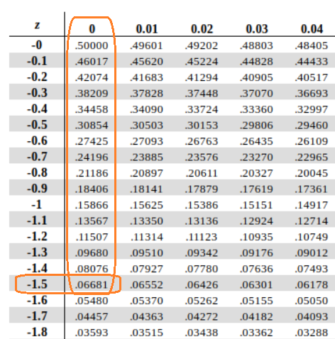
What’s nice about z-scores is that they can also be used to find proportions, which will be talked about even more in the next post. This requires the Unit Normal Table which is a table designed to help one translate z-scores into proportions of the population on either side of the score or compared to the mean score. There are 4 columns: one with the z-scores, one with the proportion of the population in the body of the distribution with the z-score as the starting point, one with the proportion of the population in the tail of the distribution with the z-score as the starting point, and one with the proportion of the population between the z-score and the mean. It can usually be found in the back of any statistics textbook. If I have a z-score of -1.5 and I wanted to know the proportion of the scores which are lower than -1.5, I could go to the back of my textbook, find -1.50 in the margins, and get the proportion .06681, meaning that 6.6881% of the data is less than a z-score of -1.5. The numbers in this table show the reader the proportion of everything to the left of the z-score in question. If I wanted to know everything to the right, the proportion would be 1 – 0.06681, which is .93319 or 93.319% of the data.

Z-scores can be used in inferential statistics. Interpretation of research results depends on determining if the (treated) sample is noticeably different from the population. The distribution of the general population would describe the average untreated person, so this allows researchers to compare that distribution to their treated sample. Z-scores are one technique for defining “noticeably different”, but it more like borders on inferential statistics, because we can’t actually tell if there’s a statistical difference without running the right test. Z-tests and their purpose in inferential statistics will be discussed in other posts.

This chapter was originally posted to the Math Support Center blog at the University of Baltimore on June 6, 2019. 

Probabilities

A probability is a fraction or a proportion of all the possible outcomes. So it’s the number of classified outcomes classified as X divided by the total number of possible outcomes (N). It’s generally reported as a decimal, but it can also be reported as a fraction or a percentage.

What is the role of probability in populations, samples, and inferential statistics? As we discussed before, because it’s usually impossible for researchers to draw data from the entirety of a population, they draw samples. The size of the sample affects how comparable the sample population is to the general population. Probability is used to predict what kind of samples are likely to be obtained from a population. Thus, probability establishes a connection between samples and populations; we know from looking at the population how likely it is for a specific sample to be drawn. We also use proportions that exist within samples to infer the probabilities that exist within a population. Inferential statistics rely on this connection when they use sample data as the basis for making conclusions about populations.

Random Sampling

Random sampling is a process by which researchers pool together a sample in such a way that it is most likely to be representative of the population as a whole. While this will never be entirely the case – since (1) there is always a chance that a sample will be entirely different from the population and (2) samples inherently always have less variability than the population – it’s good practice to follow certain random sampling requirements:

• Independent random sampling: Probabilities must stay constant from one selection to the next if more than one individual is selected. In other words, selecting one individual shouldn’t affect the probability of another person being selected; their chances are independent of one another.
• Random sampling with replacement: Each individual in the population has an equal chance of being selected, meaning that to keep the denominator of the probability equation (X/N) the same for each draw, the first draw needs to be returned to the population pool.

Proportions in Frequency Distributions

Proportions can be represented in frequency distributions, and this was briefly touched on in another blog post about z-scores. A selected section of a frequency distribution represents a proportion of the population; the selected area under the curve represents a proportion of the population. Because normal distributions are symmetrical and the same shape, just stretched out differently, we can use z-scores to standardize the scores and use a unit normal table to determine what proportion of the population is on either side of that score. The area under the curve literally becomes a proportion. We also know that in a normal distribution, more extreme scores are less likely to occur, since most scores will build up near the mean. The proportions of ranges of scores closer to the mean are greater than the proportions of scores in the ranges near the tails of the distribution.

This chapter was originally posted to the Math Support Center blog at the University of Baltimore on on June 6, 2019. 

Up until this point, as far as distributions go, it’s been about being able to find individual scores on a distribution. Moving into hypothesis testing, we’re going to switch from working with very concrete distributions with scores to hypothetical distributions of sample means. In other words, we’re still working with normal distributions, but the points that make up the distribution will no longer be individual scores, but all possible sample means which can be drawn from a population with a given or number of scores in them.

We use these kinds of distributions because with inferential statistics we’re going to want to find the probability of acquiring a certain sample mean to see if it’s common or very rare and therefore perhaps significantly different from another mean.

There are some concepts you will have to keep in mind for this shift including sampling error, the central limit theorem, and standard error.

Sampling Error

Sampling error is the natural discrepancy, or amount of error, between a sample statistic and its corresponding population parameter. So each sample is different because you’re likely drawing separate samples from the same population; you hope to get a diverse group, but you don’t really get to pick what you get, and you’re not likely to get the exact same group twice. Samples can’t be entirely representative of a population and always have less variability than the population. So even though we take a sample in order to run statistics that can be generalized back to the population, there is always going to be some error.

Central Limit Theorem

The central limit theorem is a set of rules that dictate how a distribution of sample means will look given certain criteria. For any population with mean and standard deviation , the distribution of sample means for sample size will have a mean of and a standard error of (which we will talk about more in a minute) and will approach a normal distribution as n approaches infinity. So this practically means that the distribution of sample means is almost perfectly normal in either of two conditions: the population from which the samples are selected is a normal distribution or the number of scores in each sample (also known as sample size) is relatively large (around 30 or more). The central limit theorem also mentions that as n increases, variability decreases. In other words, the greater the sample n, the pointer your distribution.

These videos will help your understanding:

Standard Error

The standard error provides a measure of how much distance is expected on average between a sample mean and the population mean . Essentially, it’s the standard deviation of sample means from the mean of sample means. It specifies precisely how well a sample mean estimates its population mean. The magnitude of the standard error is determined by two factors: the size of the sample and the standard deviation of the population from which the sample is selected. We can see by the equation that the greater is, the greater its square root and the more that the standard deviation will have to be divided by, making the standard error smaller. But if the population standard deviation is already small, that will make the standard error small too.

Inferential Statistics

Inferential statistics are methods that use sample data as a basis for drawing general conclusions about populations, and as mentioned before, are the reason why we’re learning about distributions of sample means. It’s important to know how much a sample differs from the population because we can’t draw many conclusions about the population from a sample that is very different. The error is important to keep in mind too when creating a control group. If a study with treated and untreated patients is to be generalized to the general population, you don’t just want to know if there was a significant difference between the two groups, but you want to make sure that the untreated group represents the general population.

This chapter was originally posted to the Math Support Center blog at the University of Baltimore on June 6, 2019. 

What is Hypothesis Testing?

Hypothesis testing is a big part of what we would actually consider testing for inferential statistics. It’s a procedure and set of rules that allow us to move from descriptive statistics to make inferences about a population based on sample data. It is a statistical method that uses sample data to evaluate a hypothesis about a population.

This type of test is usually used within the context of research. If we expect to see a difference between a treated and untreated group (in some cases the untreated group is the parameters we know about the population), we expect there to be a difference in the means between the two groups, but that the standard deviation remains the same, as if each individual score has had a value added or subtracted from it.

Steps of Hypothesis Testing

The following steps will be tailored to fit the first kind of hypothesis testing we will learn first: single-sample z-tests. There are many other kinds of tests, so keep this in mind.

• Step 1: State the Hypothesis
  • Null Hypothesis (H0): states that in the general population there is no change, no difference, or no relationship, or in the context of an experiment, it predicts that the independent variable has no effect on the dependent variable.
  • Alternative Hypothesis (H1): states that there is a change, a difference, or a relationship for the general population, or in the context of an experiment, it predicts that the independent variable has an effect on the dependent variable.
• Step 2: Set the Criteria for a Decision
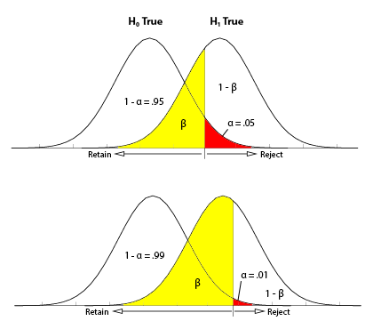
  • Alpha Level: Also known as Level of Significance, is a probability value that is used to define the concept of “very unlikely” in a hypothesis test. We chose an alpha level in order to separate the most unlikely sample means from the most likely sample means. Ex. that means that we’re separating the most unlikely 5% from the most likely 95%. The largest permissible value of alpha is 0.05, although some researchers like to use more conservative alpha levels to reduce the risk that a false report is published. But you don’t want the value to be too conservative because otherwise, you might run the risk of a Type II error, in which case the hypothesis test demands more evidence from the research results, in which case you might be throwing out evidence that a treatment will work.
  • Critical Region: Composed of the extreme sample values that are very unlikely to be obtained if the null hypothesis is true. Determined by alpha level. If sample data fall in the critical region, the null hypothesis is rejected, because it’s very unlikely they’ve fallen there by chance.
• Step 3: Collect Data and Compute Sample Statistics
  • After collecting the data, we find the sample mean. Now we can compare the sample mean with the null hypothesis by computing a z-score that describes where the sample mean is located relative to the hypothesized population mean. We use the z-score formula.
• Step 4: Make a Decision
  • We decided previously what the two z-score boundaries are for a critical score. If the z-score we get after plugging the numbers in the aforementioned equation is outside of that critical region, we reject the null hypothesis. Otherwise, we would say that we failed to reject the null hypothesis.

Regions of the Distribution

Because we’re making judgments based on probability and proportion, our normal distributions and certain regions within them come into play.

As mentioned before, Alpha Level, also known as Level of Significance, is a probability value that is used to define the concept of “very unlikely” in a hypothesis test. We chose an alpha level in order to separate the most unlikely sample means from the most likely sample means. Ex. that means that we’re separating the most unlikely 5% from the most likely 95%

The Critical Region is composed of the extreme sample values that are very unlikely to be obtained if the null hypothesis is true. Determined by alpha level. If sample data fall in the critical region, the null hypothesis is rejected, because it’s very unlikely they’ve fallen there by chance.

These regions come into play when talking about different errors.

A Type I Error occurs when a researcher rejects a null hypothesis that is actually true; the researcher concludes that a treatment has an effect when it actually doesn’t. This happens when a researcher unknowingly obtains an extreme, non-representative sample. This goes back to alpha level: it’s the probability that the test will lead to a Type I error if the null hypothesis is true.

A Type II Error occurs when a researcher fails to reject the null hypothesis that is really false; this means that the hypothesis test has failed to detect a real treatment effect. This happens when the sample mean is not in the critical region even though the treatment has had an effect on the sample. Usually, this means that the effect of the treatment was small, but it’s still there. The probability of a Type II error is represented by beta

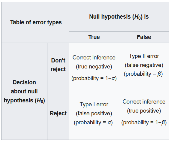
A result is said to be significant or statistically significant if it is very unlikely to occur when the null hypothesis is true. That is, the result is sufficient to reject the null hypothesis. For instance, two means can be significantly different from one another.

Factors that Influence and Assumptions of Hypothesis Testing

Assumptions of Hypothesis Testing:

• Random sampling: it is assumed that the participants used in the study were selected randomly so that we can confidently generalize our findings from the sample to the population.
• Independent observation: two observations are independent if there is no consistent, predictable relationship between the first observation and the second.
  The value of σ is unchanged by the treatment; if the population standard deviation is unknown, we assume that the standard deviation for the unknown population (after treatment) is the same as it was for the population before treatment. There are ways of checking to see if this is true in SPSS or Excel.
• Normal sampling distribution: in order to use the unit normal table to identify the critical region, we need the distribution of sample means to be normal (which means we need the population to be distributed normally and/or each sample size needs to be 30 or greater based on what we know about the central limit theorem).

Factors that influence hypothesis testing:

• The variability of the scores, which is measured by either the standard deviation or the variance. The variability influences the size of the standard error in the denominator of the z-score.
• The number of scores in the sample. This value also influences the size of the standard error in the denominator.

Test statistic: indicates that the sample data are converted into a single, specific statistic that is used to test the hypothesis (in this case, the z-score statistic).

Directional Hypotheses and Tailed Tests

In a directional hypothesis test, also known as a one-tailed test, the statistical hypotheses specify with an increase or decrease in the population mean. That is, they make a statement about the direction of the effect.

The Hypotheses for a Directional Test:

• H0: The test scores are not increased/decreased (the treatment doesn’t work)
• H1: The test scores are increased/decreased (the treatment works as predicted)

Because we’re only worried about scores that are either greater or less than the scores predicted by the null hypothesis, we only worry about what’s going on in one tail meaning that the critical region only exists within one tail. This means that all of the alpha is contained in one tail rather than split up into both (so the whole 5% is located in the tail we care about, rather than 2.5% in each tail). So before, we cared about what’s going on at the 0.025 mark of the unit normal table to look at both tails, but now we care about 0.05 because we’re only looking at one tail.

A one-tailed test allows you to reject the null hypothesis when the difference between the sample and the population is relatively small, as long as that difference is in the direction that you predicted. A two-tailed test, on the other hand, requires a relatively large difference independent of direction. In practice, researchers hypothesize using a one-tailed method but base their findings off of whether the results fall into the critical region of a two-tailed method. For the purposes of this class, make sure to calculate your results using the test that is specified in the problem.

Effect Size

A measure of effect size is intended to provide a measurement of the absolute magnitude of a treatment effect, independent of the size of the sample(s) being used. Usually done with Cohen’s d. If you imagine the two distributions, they’re layered over one another. The more they overlap, the smaller the effect size (the means of the two distributions are close). The more they are spread apart, the greater the effect size (the means of the two distributions are farther apart).

Statistical Power

The power of a statistical test is the probability that the test will correctly reject a false null hypothesis. It’s usually what we’re hoping to get when we run an experiment. It’s displayed in the table posted above. Power and effect size are connected. So, we know that the greater the distance between the means, the greater the effect size. If the two distributions overlapped very little, there would be a greater chance of selecting a sample that leads to rejecting the null hypothesis.

This chapter was originally posted to the Math Support Center blog at the University of Baltimore on June 11, 2019.

Z-tests vs. t-tests

Z-tests compare the means between a population and a sample and require information that is usually unavailable about populations, namely the variance/standard deviation. Single sample t-tests compare the population mean to a sample mean, but only require one variance/standard deviation, and that’s from the sample. This is where estimated standard error comes in. It’s used as an estimate of the real standard error, when the value of is unknown. It is computed using the sample variance or sample standard deviation and provides an estimate of the standard distance between a sample mean, , and the population mean, , (or rather, the mean of sample means). It’s an “error” because it’s the distance between what the sample mean is and what it would ideally be since we would rather have the population standard deviation. The formula for estimated standard error is .

The formula for the t-test itself is:

with the bottom portion referring to the estimated standard error. You may see this written as instead.

Degrees of Freedom

Degrees of freedom describe the number of scores in a sample that are independent and free to vary. Because the sample mean places a restriction on the value of one score in the sample, there are degrees of freedom for a sample with n scores. For a single sample t-test, the degrees of freedom are calculated using the following formula: .

Shape of a t-distribution

One general rule of t-distribution is that it’s always slightly flatter than it’s corresponding normal distribution. This is because t-statistics are always working from a sample size, which is relatively small, rather than a population, which are generally large.

There are some factors which also influence the shape of each individual t-distribution:

• The degrees of freedom: The greater n is, and subsequently df, the more like a normal distribution the t-distribution will begin to look (this also follows the 30 rule)
• The sample variance: The bottom half of the equation deals with the estimated standard error, which changes when the standard deviation changes. Because the ESE is dependent on the sample variance, each sample can create a different ESE

Hypothesis Testing with a Single Sample t-test

The written null and alternative hypotheses for a single sample t-test are as follows:

H0 : = population mean

H1 : \neq population mean

The stops for a single sample t-test are as follows:

1. State the hypotheses and select an alpha level
2. Locate the critical region
3. Calculate the test statistic
4. Make a decision regarding the null hypothesis

The following are some assumptions one makes when doing a single sample t-test:

• The values in the sample must consist of independent observations.
• The population that is sampled must be normal.

Effect Size for Single Sample t-tests

Effect size for a single sample t-test is calculated using Cohen’s d. The formula for this is the mean difference over the standard deviation, or . Effect size is important because it’s a way of quantifying the difference between two groups, rather than just saying that there is a significant difference. Essentially, it’s also important to know how much of a difference there is, not just the likelihood that the group differences you’re seeing are a fluke because the null hypothesis is actually true. This can also be important for practical significance. If your treatment is statistically significant, but has a small effect size, is it worth using this treatment on clients?

For Cohen’s d, 0.2 would be considered a small effect size, 0.5 is medium, and 0.8 is large. Some people will mix words together like “small to medium effect size” but some professors will want you to just pick a side.

Confidence Intervals

Confidence intervals are a range of values which is likely to encompass the true value you’re looking for. More specifically, it’s a range we create using a sample that we can say with X% confidence that the population mean falls within that range. Confidence intervals are constructed at a confidence level, such as 95%, selected by the user. It means that if the same population is sampled on numerous occasions and interval estimates are made on each occasion, the resulting intervals would bracket the true population parameter in approximately 95% of the cases. Confidence intervals and any kind of interval estimation are used in the same situations that you would use hypothesis testing. There is an estimation procedure for every kind of hypothesis test.

This chapter was originally posted to the Math Support Center blog at the University of Baltimore on June 11, 2019.

We have talked about single sample t-tests, which is a way of comparing the mean of a population with the mean of a sample to look for a difference. With two-sample t-tests, we are now trying to find a difference between two different sample means. More specifically, independent t-tests involve comparing the means of two samples which are distinctly different from one another in regards to the individuals within each sample. For example, a group of pet owners vs. a group of folks who don’t own pets. These two groups are completely independent of one another. This distinction will be important in a later post.

A more technical explanation of the difference between a single sample and two-sample is that a single sample t-test revolves around drawing conclusions about a treated population based on a sample mean and an untreated population mean (no standard deviation). An independent sample t-tests are all about comparing the means of two samples (usually a control group/untreated group and a treated group) to draw inferences about how there might be differences between those two groups in the broader population

There are some distinct advantages and disadvantages to this approach when compared to other approaches. To avoid confusion, we won’t describe the other approaches here but will just mark the advantages and disadvantages of this one here for your consideration:

Advantages:

• Gives the opportunity to conduct an experiment with very little contamination by extraneous factors.
• Lowers the chance of participants suffering from boredom after a long series of tests as well as skewing the results by becoming more accomplished through practice experience.

Disadvantages:

• Can be complex.
• Requires a large number of participants.
• Needs a new group for every treatment and manipulation.
• Confounding variables brought in by the individuals in the study can weaken results.

Hypothesis Testing with Independent t-tests

The null and alternative hypotheses for this kind of test are as follows:

(no difference in the population means)

(there is a mean difference)

Steps of calculating an independent samples t-test (from this point forward, if there is a larger formula you’re looking for, see our formula guide glossary):

1. Calculate the estimated standard error by calculating pooled variance and figuring out the degrees of freedom for each group.
2. Subtract the two means from one another (we assume that the difference between the population means will be 0 given the null hypothesis) and then divide by the standard error.
3. Determine the critical region based on your alpha level and whether you’re running a one or two-tailed test. Then decide whether your calculated t-test falls within the critical region or not.
4. Make a decision about the null hypothesis based on this comparison.

Assumptions of independent sample t-tests:

• The observations within each sample must be independent.
• The two populations from which the samples are selected must be normal.
• To justify using the pooled variance, the two populations from which the samples are selected must have equal variances (homogeneity of variance); essentially the standard deviation of after treatment should be very similar to the standard deviation presented before treatment. This can be confirmed using SPSS or Excel. This can also be done using Hartley’s F-max test, which is described later on in this chapter.

Estimated Standard Error and Pooled Variance

To calculate the estimated standard error, you need to first calculate pooled variance, especially because not all treatment or non-treatment groups will have the same number of scores, and so you need to weight in both groups before coming to terms with the overall estimated standard error. Remember that the estimated standard error is how we calculate the standard error when there’s no population mean to go off of.

In essence, the steps for calculating a t-test by hand are:

1. Find the sum of squares of each sample.
2. Calculate the pooled variance given the sums of squares you just found and the degrees of freedom ( for each sample).
3. Calculate the estimated standard error using that pooled variance.
4. Plug the estimated standard error into the t-test formula and solve for .

Effect Size of Independent Samples t-test

We use Cohen’s d to get effect size. For this particular test, it’s mean 1 minus mean 2 all divided by the square root of the pool variance calculated earlier. In this case, instead of comparing the effects of a sample to the population (asking, is this practically significant rather than just statistically significant?), we’re comparing the effects of two different samples.

Hartley’s F-Max Test

Hartley’s F-max test is a statistical test to evaluate the homogeneity assumption. To compute, you need to compute the sample variance of each sample individually. Then, you need to make a fraction with the biggest variance on top and the smallest one on the bottom. Finally, compute. The F-max value computed for the sample data is compared with the critical value found in an F-max table. If the sample value is larger than the table value, then you can conclude that the homogeneity assumption is not valid.

If you’re looking for more help on learning the concept of the independent samples t-test or how to calculate it, check out this series of videos (each one about five minutes long):

This chapter was originally posted to the Math Support Center blog at the University of Baltimore on June 11, 2019.

A repeated measures or paired samples design is all about minimizing confounding variables like participant characteristics by either using the same person in multiple levels of a factor or pairing participants up in each group based on similar characteristics or relationship and then having them take part in different treatments. Matched subjects is another word used to describe this kind of test and it is used specifically to refer to designs in which different people are matched up by their characteristics. Participants are often matched by age, gender, race, socioeconomic status, or other demographic features, but can also be matched up on other characteristics the researchers might consider possible confounds. Twin studies are a good example of this kind of design; one twin has to be matched up with the other – they can’t be matched to someone else’s twin.

To reiterate the differences between a repeated measures t-test and the other kinds of tests you may have learned up to this point, a single sample t-test revolves around drawing conclusions about a treated population based on a sample mean and an untreated population mean (no standard deviation). An independent sample t-tests are all about comparing the means of two samples (usually a control group/untreated group and a treated group) to draw inferences about how there might be differences between those two groups in the broader population. Different, randomly assigned participants are used in each group. Related samples t-tests are like independent sample t-tests except they use the same person for multiple test groups or they match people based on their characteristics or relationships to cut down on extraneous variables which may interfere with the data.

Mean Difference and Estimated Standard Error of the Mean Difference

The mean difference is calculated by subtracting the two scores collected from each person (because there are two testing groups), adding all of those differences up, and then dividing that number by the number of scores. This is done because rather than just compare means between the two samples, like in an independent samples t-test, we have the opportunity to first calculate the difference between each individual to see how the treatment affected them.

The estimated standard error of the mean difference is a measure of how much the mean difference might vary from one occasion to the next. This is different from independent measures because instead of pooling variance between two samples, you base your sum of squares on the difference between the two scores and then calculate the estimated standard error like you would a single sample t test.

Hypothesis Testing with Repeated Measures t-tests

The null and alternative hypothesis are written as follows:

or that there is no difference between the two conditions

or that there is a significant difference between the two conditions

Steps for calculating a repeated measures t-test (all formulas needed can be found in the statistics formula glossary):

1. State the null and alternative hypothesis
2. Locate the critical region (remember that the is )
3. Calculate the t statistic using the t formula after calculating the estimated standard error of the mean difference.
4. Make a decision.

Once again, there are some advantages and disadvantages to using this approach.

Advantages:

• Fewer subjects needed
• Is well-suited for studying changes over time (developmental, learning, studying)
• Reduces or eliminates caused by individual differences within the participants by either linking participants up based on characteristics or by using the same person twice.

Disadvantages:

• Increases the likelihood that outside factors that change over time may be responsible for changes in the participants’ scores.
• Participation in the first treatment could affect scores in the second treatment (practice, fatigue, etc.).

Effect Size for Repeated Measures t-tests

Once again, Cohen’s d is the effect size measurement of choice. In this case, it’s the sample mean difference over the sample mean deviation (so whatever you found as the variance, square root that to get the sample mean deviation).

Variability as a Measure of Consistency

If a treatment consistently adds a few points to each individual’s score, then the set of difference scores are clustered together on a normal distribution curve with relatively small variability. In this situation, with small variability, it is easy to see the treatment effect and it is likely to be significant. High variability means that there’s no consistency with a treatment effect, meaning that it’s harder to see that there’s any difference between groups and it’s unlikely that a significant difference will be found.

Degrees of Freedom

Before, when we were working with independent t-tests, the degrees of freedom was for each sample, so in the end, it was . However, for a repeated measures t-test, we’re only needing degrees of freedom for the mean difference. Therefore, the total degrees of freedom is simply .

This chapter was originally posted to the Math Support Center blog at the University of Baltimore on June 11, 2019.

An ANOVA (ANalysis Of VAriance) is a test that is run either to compare multiple independent variables with two or more levels each, or one independent variable with more than 2 levels. You can technically also run an ANOVA in the same cases you would run a t-test and come up with the same results, but this isn’t common practice, as t-tests are easier to compute by hand.

For the purposes of this post, a One-way ANOVA is a test which compares the means of multiple samples (more than 2) which are connected by the same independent variable. An example of this might be comparing the growth of plans who receive no water (Group 1) a little water (Group 2), a moderate amount of water (Group 3), and a lot of water (Group 4).

A factor is another name for an independent variable. As mentioned earlier, ANOVAs can sometimes have more than one factor, but for now we’re only working with one, just like we have before. A level is a group within that independent variable. Using the example from before, the groups in which the plants are put in are the levels (no water, little water, some water, a lot of water) and the independent variable itself is just water amount.

Experiment-wise Alpha

A question you might be asking yourself is, why bother doing an ANOVA when I can just do multiple t-tests? This is because the risk of a Type I error that accumulates as you do more and more separate tests. Doing multiple t-tests would result in greater experiment-wise alpha and therefore experiment-wise error. In a lot of ways its better to just do one big ANOVA to look for differences and then decipher those differences later using a post-hoc, which will be discussed later.

Hypothesis Testing with One-way ANOVAs

The null and alternative hypotheses for a one-way ANOVA are as follows (please keep in mind that 3 is not the maximum number of means that can be compared so write your hypotheses accordingly):

Essentially, the point is whether there will or won’t be a significant difference between the groups, or at least two of them.

Steps for calculating a one-way ANOVA (please refer to the statistics formula glossary for actual formulas):

Variability in One-Way ANOVAs

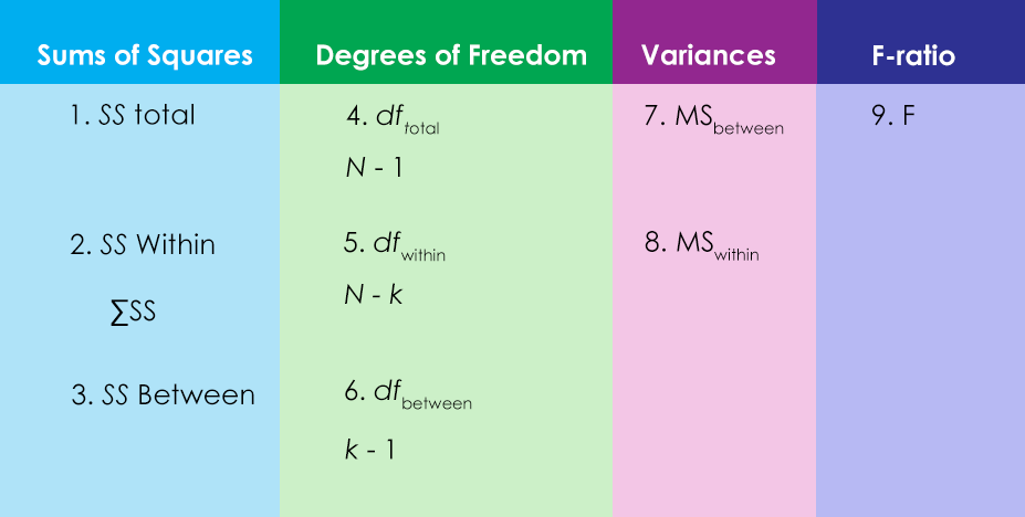
There are multiple kinds of variability found within the calculation of an ANOVA. There is between-treatment variance and within-treatment variance. The between-treatment variance can be further broken down into systematic treatment effects and random, unsystematic factors. The within-treatment variance only accounts for random, unsystematic factors in this case.

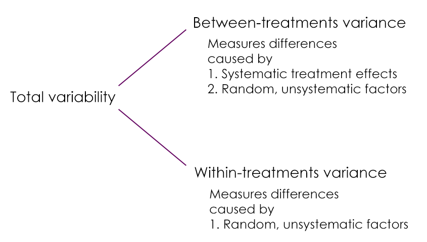
The purpose of calculating within-treatments variance is to determine how much of the between-treatment variance was due to random, unsystematic factors and how much was due to treatment effects.

There is a conceptual meaning underlying the ANOVA formula. The numerator is meant to represent the differences between sample means and the denominator is meant to represent the differences between samples expected with no treatment effect. This is basically between-treatments variance (the general differences between treatment conditions) and within-treatment variance (the variability within each sample).

Assumptions of a one-way ANOVA

• The observations within each sample must be independent.
• The population from which the samples are selected must be normal.
• The populations from which the samples are selected must have equal variance (homogeneity of variance).

Effect Size in One-Way ANOVAs

Effect size is now calculated with something called partial eta squared. The formula for this is: , or the sum of squares of the between treatments over the sum of squares total.

Post-Hoc Test

A post-hoc test allows one to figure out which groups are significantly different from one another once a significant F-ratio has been established. This is better than just running individual t-tests because post hoc still reduce experiment-wise error. There are several options for conducting a post-hoc, but two more popular options are Tukey’s and Scheffe’s tests. Tukey’s test calculates a single value that determines the minimum difference between treatment means that is necessary for significance. Scheffe’s test uses an F-ratio to evaluate the significance of the difference between the two treatment conditions. Formulas for both of these tests are in the statistics formula glossary.

This chapter was originally posted to the Math Support Center blog at the University of Baltimore on June 11, 2019.

Just like when we talked about independent samples t-tests and repeated measures t-tests, ANOVAs can have the same distinction. Independent one-way ANOVAs use samples which are in no way related to each other; each sample is completely random, uses different individuals, and those individuals are not paired in any meaningful way. In a repeated measures one-way ANOVA, individuals can be in multiple treatment conditions, be paired with other individuals based on important characteristics, or simply matched based on a relationship to one another (twins, siblings, couples, etc.). What’s important to remember that in a repeated measures one-way ANOVA, we are still given the opportunity to work with multiple levels, not just two like with a t-test.

Advantages:

• Individual differences among participants do not influence outcomes or influence them very little because everyone is either paired up on important participant characteristics or they are the same person in multiple conditions.
• A smaller number of subjects needed to test all the treatments.
• Ability to assess an effect over time.

Disadvantages:

• Increases the likelihood that outside factors that change over time may be responsible for changes in the participants’ scores.
• Participation in the first treatment could affect scores in the second treatment (practice, fatigue, etc.).

Hypothesis Testing with Repeated Measures One-Way ANOVA

The null and alternative hypotheses for a repeated measures ANOVA are as follows:

Assumptions of repeated measures one-way ANOVAs are as follows:

• The observations within each treatment condition must be independent.
• The population distribution within each treatment must be normal
• The variances of the population distribution for each treatment should be equivalent

The steps to calculating a repeated measures one-way ANOVA are explained in this chart.

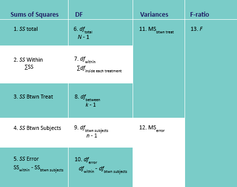
See below for a useful video. Please remember that different disciplines use different versions of the same equations; don’t let this intimidate you. Just use what you have been given by your book or professor.

A YouTube element has been excluded from this version of the text. You can view it online here: https://ubalt.pressbooks.pub/mathstatsguides/?p=231

There is a conceptual meaning underlying the process of calculating this. There are more sums of squares to consider because we’re doing our best to separate within differences from between differences but also distinguishing which within differences are due to individual differences between the subjects and what error can’t be accounted for by individual differences. So instead of basing an F-ratio on the balance of between treatment differences and any error that could ever take place, we reduce the error being used to calculate whether there’s a significant difference by getting rid of the kind of error we can measure with a repeated measures design: participant differences. See the graphic below for a visual representation of this concept.

Effect Size

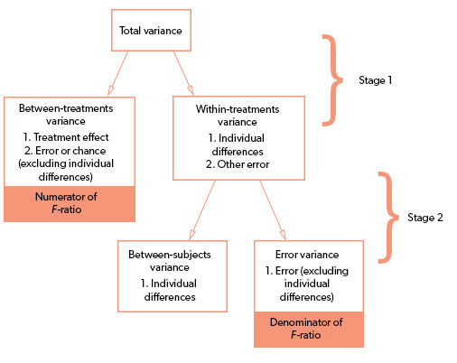
Effect size, in this case, is calculated once again using partial eta squared:

Be careful not to accidentally plug in the wrong value, as these names all sound similar to one another. The numerator should be the between treatments sum of squares gotten in the first step of the calculation. The denominator is the total sum of squares minus the between-subjects sum of squares found in the second round of calculations.

Post Hoc Tests

Like we mentioned in the previous post, post hoc tests are tests run to determine which groups are significantly different from one another after determining through the ANOVA that there’s a significant difference somewhere. Is the significant difference between A and B, B and C, C and A, or all three? For repeated measures one-way ANOVAs, Tukey’s HSD and Scheffe can be used, just substitute SSerror and dferror in the formulas. These formulas can be found on the statistics formula glossary post.

This chapter was originally posted to the Math Support Center blog at the University of Baltimore on June 18, 2019.

So far we’ve talked about tests which are used if there is one independent variable, either with two levels or more. This is not the limit of how much we can include in a single analysis. In a two-factor ANOVA, there is more than one independent variable and each of those variables can have two or more levels. Take this example into consideration:

A farmer wants to know the best combination of products to use to maximize her crop yield. She decides to test out three different fertilizer brands (A, B, and C) and two different kinds of seeds (Y and Z). Each product is paired once with another for a total of 6 conditions: AY, BY, CY, AZ, BZ, CZ.

A two-factor ANOVA considers more than one factor and considers the joint impact of factors. This means that instead of running a new study every time you want to see how an independent variable affects a specific dependent variable, you can run an experiment with two different independent variables and seeing how they each impact the dependent variable and you get to see if the two independent variables do anything together to affect the dependent variable. These are called main effects and interactions. Keeping the example going, if we find that no matter what the seed type is that fertilizers A, B, and C resulted in different crop yields from one another, we would say there is a main effect for fertilizer type. If no matter what the fertilizer type is there is a difference between the crop yields of seeds Y and Z, we would say that there is a main effect for seed type. If there are times that the two factors influence each other (for example, let’s say that fertilizer worked much better specifically when paired with Y seeds), we would say there’s an interaction. The defining characteristic of an interaction is when the effect of one factor depends on the different levels of a second factor or the impact of another factor, either amplifying or reducing the effect based on the level.

Meaning of the Equation Before the ANOVA

Often times when reading a paper which uses a multiple factor ANOVA, there is a little equation before it like 2×2 or 4x5x2 or something along those lines. These equations may look confusing and intimidating, but there is a simple way to read these. The number of numbers in the equation tells you how many factors there are. For instance, a 2×3 ANOVA simply has two factors because there are only two numbers presented. A 4x5x7x2x3x4 ANOVA, although this equation looks ridiculous, simply has six factors in it because there are six numbers present. The actual values of each number tell you how many levels are in each factor. A lot of papers make sure to define which factors they’re considering first, but simply put, a 2×3 ANOVA has two factors and the first factor has two levels while the second has three. A 4x5x7x2x3x4 ANOVA has six factors, the first has four levels, the second has five, the third has seven, the fourth has two, the fifth has three, and the sixth has four. This author has personally never come across an ANOVA so convoluted in a paper, but this example was just meant to show that although it’s easy to get caught up in the sheer volume of numbers, interpreting them is not so complicated. Also remember that it’s the author’s job in an article to interpret the results for you, so that should help.

Hypothesis Testing with Two-Factor ANOVAs

For an ANOVA with only two factors (which is all you’ll likely need to master), there are three different null and alternative hypotheses to consider. One is for the first main effect, one is for the second main effect, and one is for an interaction. Don’t forget to include as many means as there are levels.

Null:

H0: There is not an A X B interaction

Alternative:

H1: There is an A X B interaction

The following are the steps and stages needed to calculate a two-factor ANOVA. Please keep in mind that the formulas needed for these calculations exist in the statistics formula glossary post.

• First Stage:
  • Is identical to independent samples ANOVA
  • Compute the , , and
• Second Stage:
  • Calculate , , , , , and .
• Third Stage:
  • The goal is to partition the into three separate components
  • Calculate , , and . In other words, calculate the parts of which can be attributed to main effect one, main effect two, and an interaction.
• Fourth Stage:
  • Calculate , , , and .
• Fifth Stage:
  • Calculate , , and
  • These are the numbers which you use to determine if there is a main effect one , main effect two , and/or an interaction .
• Sixth Stage:
  • If there is a significant main effect that has three or more levels, this is when you would conduct a post-hoc analysis for that factor alone. This would be no different than one done for a one-way ANOVA.

The conceptual meaning behind these calculations is that we’re dividing up the variance between the treatments so that we know the differences between the levels of factor A, the differences between the levels of factor B, and then the differences due to an interaction between the factors.

The assumptions of a two-factor ANOVA are as follows:

• The observations within each sample must be independent of each other.
• The populations from which the samples are selected must be normally distributed.
• The populations from which the samples are selected must have equal variances.

Effect Size

Once again we’re using partial eta squared, but this time we’re calculating it thrice – once for main effect one, once for main effect two, and once for an interaction. The formulas for these are relatively simple and can be found in the statistics formula glossary post.

This chapter was originally posted to the Math Support Center blog at the University of Baltimore on June 18, 2019.

So far we’ve been talking about analyses which involve variables which are split up into categorical or discrete variables (ex. treatment A, B, C) compared to a dependent variable which is continuous (ex. plant height). However, there is a way to look at two variables which have continuous data: correlation. A correlation will tell you the characteristics of a relationship such as direction (either positive or negative), form (we often work with linear relationships), and strength of the relationship. Strength and direction can be understood with the number which is given at the end of an analysis .

A positive correlation is one in which the increased value of one variable results in the increased value of another. For example, height and weight – as height increased, weight also tends to increase. A negative correlation is one in which the increased value of one variable results in the decrease of another. For example, as the temperature outside increases, hot chocolate sales will decrease. This is what is meant by the direction of a correlation. An r-value with a negative sign in front of it means a negative correlation and one without a negative sign means a positive correlation.

R-values exist on a plane between -1 and 1. The closer a number is to 1, the stronger its positive relationship. The closer a number is to -1, the stronger its negative relationship. The closer a number is to 0, the weaker its relationship, no matter if its negative or positive.

Created by Spiritia and shared under a CC BY-SA 3.0 License

Pearson Correlation

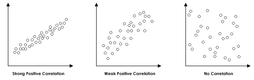
The most common type of correlation used is the Pearson Correlation. It measures the degree and direction of the linear relationship between two variables. It will measure a perfect linear relationship. Every change in variable has a corresponding change in variable . The possible range of an r-value is between -1 and 1. is calculated in the following way: = covariability / variability of and separately.

There are some important factors to take into consideration when using and interpreting the Pearson Correlation.

1. Correlation does not demonstrate causation. This is something very important to remember; just because two variables have a correlation doesn’t mean that one is causing the other. There may be another factor that we haven’t measured which may be the real reason. Take into account that when ice cream sales go up, so do the number of drownings in an area. Does that mean that ice creams are causing people to drown? Consider that maybe increased temperatures result in more ice cream consumption as well as an increase in the number of people who are going out swimming. You can never know if there’s a third lingering factor with just a correlation.
2. The value of the correlation is affected by the range of scores in the data. For example, if you’re looking at how height and age correlate, if your sample is just made up of people who are 20 or older, you probably will get a weak correlation, as most adults no longer grow. However, if your sample is 17 or younger, you’re likely to find a decent positive correlation.
3. Extreme points (outliers) have an impact. Data points which vary greatly from the others may sometimes need to be removed as their presence affects the correlation.
4. Correlation cannot be interpreted as a proportion.

Coefficient of Determination

The coefficient of determination is a measurement of the proportion of variability in one variable that can be determined from the relationship with the other variable (r squared). In other words, it’s used to analyze how differences in one variable can be explained by a difference in a second variable. The example given by Statistics How To is that when you get pregnant has a direct relation to when they give birth. Link to the whole article here. This measure is usually reported along the lines of this: “75% of the variation in can be explained by the variation in .”

Other Types of Correlation

While Pearson Correlation is the most commonly used, there are times when the data one collects warrants the use of a different kind of correlation. Some are listed below:

• Partial correlation: A partial correlation measures the relationship between two variables while controlling the influence of a third variable by holding it constant.
• Spearman correlation: Used when both variables are measured on an ordinal scale; Used when the relationship is consistently directional but may not be linear.
• Point-biserial correlation: Measures relationship between two variables when one variable has only two values (dichotomous value)
• Phi-coefficient: Both variables are dichotomous. Both variables are re-coded to values 0 and 1

This chapter was originally posted to the Math Support Center blog at the University of Baltimore on June 18, 2019.

Linear regression is a method for determining the best-fitting line through a set of data. In a lot of ways, it’s similar to a correlation since things like and are still used. The one difference is that the purpose of regression is prediction. The best-fitting line is calculated through the minimization of total squared error between the data points and the line.

The equation used for regression is or some variation of that. If you remember from algebra class, this formula is like . This is because they are both the linear equation. Although you may be asked to report and , the purpose of regression is to be able to find values for the slope and the y-intercept that creates a line that best fits through the data.

Standard Error of the Estimate

Regression equations make a prediction, and the precision of the estimate is measured by the standard error of the estimate. The standard error of the estimate is a measure of the accuracy of predictions made with a regression line and has to do with how wide the data points are scattered (strength of the correlation). In other words, it tells you how far away the points tend to be from the prediction line.

Here is a playlist of videos that may be helpful:

A YouTube element has been excluded from this version of the text. You can view it online here: https://ubalt.pressbooks.pub/mathstatsguides/?p=244

This chapter was originally posted to the Math Support Center blog at the University of Baltimore on June 18, 2019.

Discrete versus Continuous Variables

A discrete variable typically originates from a counting process while a continuous variable usually comes from a measuring process. An easy way to make the distinction between a discrete and a continuous variable is that discrete variables are usually whole numbers with no decimals. Continuous variables on the other hand frequently take the form of decimals. For instance, the number of people which exist within a group is a discrete variable because it’s always a whole number, while a person’s weight would be continuous since it can typically be measured to multiple decimal places.

The Probability Distribution for a Discrete Variable

A probability distribution for a discrete variable is simply a compilation of all the range of possible outcomes and the probability associated with each possible outcome. Since, probability in general, by definition, must sum to 1, the summation of all the possible outcomes must sum to 1. For example, if you’re flipping a coin once, there’s a 1 in 2 chance it will land on heads, and a 1 in 2 chance it will land on tails; 1/2 + 1/2 = 1. In this way, measuring probability is similar to the use of percentages. Percentages are always measured out of 100 while probability is always measured out of 1. This is true for all probability measurements.

Expected Value for a Discrete Variable

The expected value for a discrete variable is essentially the same as the population mean. In this way, the expected value is calculated simply by finding the product of each possible outcome and its associated probability and doing a summation at the end.

Standard Deviation and Variance of a Discrete Variable

Standard deviation is basically a measure of how much each data point varies away from the mean; it’s also often described as the spread of the distribution. Quantitatively, the standard deviation is simply the square root of variance. This quantitative definition confirms the fact that variance must always be a positive number since numerically the evaluation of standard deviation would be impossible otherwise. Conversely, the standard deviation can be both positive and negative as each data point can be both above and below the mean value. Standard deviation and variance as concepts are also discussed in an earlier post called Basics of Variability.

Binomial Distribution

The binomial distribution is a type of mathematical model. Mathematical models allow us to easily calculate the probability of occurrence of any specific value of the variable of interest. The binomial distribution is used in situations where the discrete variable is the number of occurrences in a sample of n observations.

There are 4 properties of the Binomial Distribution:

1. The sample must consist of a fixed number of observations,
2. Each and every observation can be categorized into one of two mutually exclusive and collectively exhaustive categories
3. The probability of an event of interest, , is constant across all observations. Therefore the probability of a non-event of interest, (sometimes called ) is constant for all observations.
4. Observations are all independent. This simply means the probability of occurrence of any observation is not dependent on any other observation.

The Binomial distribution formula:

And

= probability that events of interest, where and are as follows:

= number of observations

= probability of an event of interest (prob.of success)

= probability of not having an event of interest (prob. of failure)

= number of events of interest (no. of successes) in the sample ( = 0,1,2, …, )

= The number of combinations of events of interest out of observations. This calculation does not take into account the order in which the events actually occur. If the order was important, that would involve calculating a permutation, not a combination. Here is a video depicting the calculation of combinations:

A YouTube element has been excluded from this version of the text. You can view it online here: https://ubalt.pressbooks.pub/mathstatsguides/?p=264

Another version of this formula which may be easier to read can be found in the Statistics Formula Glossary.

When conducting calculations for binomial distributions, there are three distinct possibilities that may be encountered.

Example: There are 10 golf balls in a bag, consisting of 6 orange balls and 4 yellow balls. If we define success as the likelihood of picking an orange ball and therefore failure as not picking an orange ball (and therefore picking a yellow ball), we can illustrate the three distinct possibilities that may be encountered in calculations.

If 6 golf balls are to be selected at random (without replacement):

• What is the probability of picking exactly 4 orange balls?

And

= probability that events of interest, when and

= number of observations = 6

= probability of an event of interest = 6/10 = 0.6

= prob. of not having an event of interest = 0.4

= number of events of interest (no. of successes) in the sample ( = 0,1,2, …, ) = 4

• What is the probability of picking at least 4 orange balls?

This equates to: prob. of 4 orange + prob. of 5 orange + prob. of 6 orange

• What is the probability of picking less than 4 orange balls?

This equates to: prob. of 0 orange + prob. of 1 orange + prob. of 2 orange + prob. of 3 orange

Prob. of at least 4 orange balls

Mean of the Binomial Distribution

The mean, ℳ, of the binomial distribution is the product of the sample size, , and the probability of an event of interest (success), .

ℳ

This is the value that is statistically most likely to occur. For instance, consider the example of tossing two unbiased dice, the range of values that may result extends from 2 to 12. The mean value is actually 7. This is because there are six distinct ways to get a value of 7. They are 1& 6, 6 & 1, 2 & 5, 5 & 2, 3 & 4, and 4 & 3. This represents 6 distinct possibilities out of a total of 36 possibilities, which is the most likely result to occur from all the distinct possibilities.

Standard Deviation of the Binomial Distribution

The standard deviation of the binomial distribution, , is the square root of the variance.

Poisson Distribution

The Poisson distribution is another type of mathematical model. The Poisson distribution applies when we want to determine the number of occurrences of a particular event in some fixed interval of time and space. This fixed interval of time and space is often called an area of opportunity. Within the area of opportunity, there can be multiple occurrences of an event.

There are 4 properties of the Poisson Distribution:

1. The area of opportunity must be defined by time, length, surface area etc. Per the Poisson distribution, we can determine the number of times a particular event occurs in a given area of opportunity.
2. The probability that an event occurs in a given area of opportunity must be the same for all the areas of opportunity.
3. The number of events that occur in each and every area of opportunity is independent of the number of events that occur in any area of opportunity
4. The probability that two or more events will occur in any area of opportunity approximates to zero as the area of opportunity becomes smaller.

The Poisson distribution formula:

where

= probability that events in an area of opportunity given

= expected number of events per unit

= mathematical constant approximated by 2.71828

= number of events ()

Example: Imagine that the mean number of cars that pass an intersection in a 1-minute interval is 5.0.

• What is the probability that in a given minute, exactly four cars will arrive?

• What is the probability that more than four cars will arrive in a given minute?

The probability that more than four cars will arrive:

4) = P (X = 4) + P (X = 5) + P (X = 6) + \cdots +" title="Rendered by QuickLaTeX.com" height="22" width="512" style="vertical-align: -6px;">

Since all probabilities in a distribution sum to 1:

4) = 1 - P(X <= 4)" title="Rendered by QuickLaTeX.com" height="22" width="261" style="vertical-align: -6px;">

Some of the material in this post was obtained from Statistics for Managers: Using Microsoft Excel, Eighth Edition.

This chapter was originally posted to the Math Support Center blog at the University of Baltimore on July 1, 2019.

Evaluating Normalcy

Many statistical tests run on the assumption that the data with which you are working is normally distributed, so it’s important to check. There are several different ways to go about this. This post will explain a few different methods for testing normalcy as well as provide some instructions about how to run these tests in Excel.

Mean vs. Median

An important rule to note about distribution is that in a normal distribution, the mean, median, and mode are approximately equal. What it looks like visually is that the mean, median, and mode are all sitting at the top of the hump of the bell curve. When a distribution is skewed, these values become different. The mode will always sit around the hump of a distribution (because this is where most of the values have accumulated). The mean is the measure of central tendency most affected by extreme variables and outliers, so it will follow the longest tail. The median, in this case, will always fall somewhere between the median and the mode. Put another way, if the distribution is positively skewed, the mean will be the greatest value, the median will be the second greatest value, and the mode will be the smallest value. If the distribution is negatively skewed, the mean will be the smallest value, the median will be the second smallest value, and the mode will be the greatest value. So when you’re looking at a data set, you may be able to get an idea of the skew of the distribution by comparing the mean and the median.

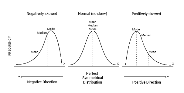
The easiest way to get all of the descriptive statistics you need in Excel is to download Analysis ToolPak. To do this go to: File>Options>Add-ins>Analysis ToolPak. Make sure to then hit GO in the bottom right, and then click the check-mark next to Analysis ToolPak before hitting OK. These directions are good for PC, but Mac users may need to find a different route for including Add-ins.

Once there, go to Data>Data Analysis. From there, you should see this pop-up.

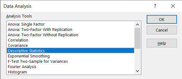
From there, click Descriptive Statistics, select your input range, select an output range, click Summary Statistics, and then click OK.

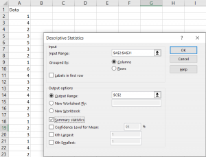
Your output should look something like this. You should be able to see the mean, standard deviation, median, mode, range, minimum, maximum, etc. These will all be helpful in future normalcy tests.

Range and Interquartile Range vs Standard Deviation

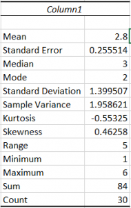
Another two questions which should be asked when comparing mean and median are, “Is the range approximately six times the standard deviation?” and “Is the interquartile range approximately 1.33 times the standard deviation?” Given the descriptive statistics we just ran, the first question should be easy to answer. Simply multiply the standard deviation by 6 and check to see if it is close to the range. Interquartile range is the difference between the first quartile and the third quartile, which are not given to you when you run the descriptive statistics. One way to find the first and third quartiles is by using the =QUARTILE function. When using this function, highlight the data, punch in a coma, and then put in the number quartile that you are interested in (1 or 3). It should look like this: =QUARTILE(A2:A:20,1). Find the difference between the two and compare this to the standard deviation multiplied by 1.33. If either of these results show wildly different results than expected, you should consider that the data may be skewed.

Boxplot

A boxplot is a quick way to see if the data you’re working with are symmetrical. To create a boxplot in Excel, highlight your data and go to Insert >Recommended Charts > All Charts > Box & Whisker. If the plot looks to be symmetrical, your data are likely normal. If one of your box sides or whiskers stretch out farther than the rest, your data may be skewed. More specifically, if your whisker extends out in the direction of the larger numbers, your data are positively skewed. If your whisker extends out to the smaller numbers, your data are negatively skewed. Below is an example of each.

Histogram

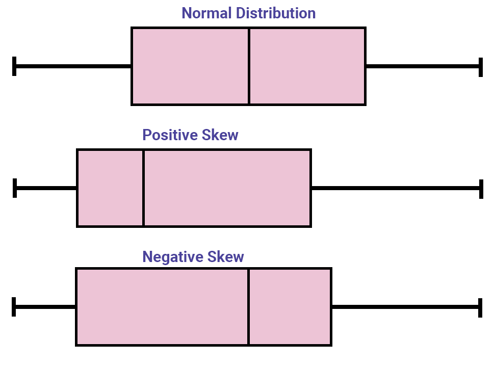
Histograms are a good way to visually check the normalcy of large amounts of data. When evaluating it, the shape of the bars should represent a bell-curve. If not, then the data may be skewed or multimodal. To create a histogram, highlight your data and go to Insert > Recommended Charts > All Charts >Histogram. When you first create the histogram, it may look a little wonky. To fix this, click the new chart, and a green plus sign should appear. Click this, hover over Axes, and move your cursor to the right until a black arrow appears. Click this, then click More Axis Options, and a bar should appear on the right side of your screen which will allow you to adjust your bin width and bin number.

Empirical Rule

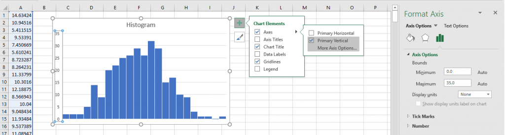
Although there is no simple way to use the empirical rule to test to see if your data are normally distributed, if you did want to take that route, the rules are as follows:

• Two-thirds of the data lie within ±1 standard deviations of the mean
• Four-fifths of the data lie within ±1.28 standard deviations of the mean
• 19 of every 20 data points lie within ± 2 standard deviations of the mean

If one were to do this in Excel, one might create a frequency distribution with these standard deviations as the bins and compare those frequencies with these rules. This can be done using the Histogram feature of Data Analysis.

Normal Probability Plot (Q-Q Plot)

A normal probability plot (otherwise known as a quantile-quantile or Q-Q plot) is a way to visualize data normalcy. Steps on how to create one in Excel are as follows:

• Step 1: Order the data from least to greatest
• Step 2: Find the expected quantile z-scores. This is done using the following equation: where is the number of data points and is the ordered value. The smallest number would have an ordered value of 1, the second smallest would have an ordered value of 2, and so on and so forth.
• Step 3: Finally, you can highlight the data and the z-scores (make sure the two columns are next to each other), go to Insert, and create a scatterplot with the data. If the line is straight, then the data is normally distributed. If the line curves upward, the data is positively skewed. If the line curves downward, the data is negatively skewed.

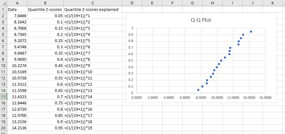
This chapter was originally posted to the Math Support Center blog at the University of Baltimore on February 4, 2020. 

This chapter includes a glossary of formulas that may be helpful to keep around when practicing statistical problems for homework or studying for an upcoming test.

PDF version: Stats-Formula-Glossary-7_16_2019

Word (.docx) version: Stats-Formula-Glossary-7_16_2019

Please keep in mind that although these formulas work, they may not be the versions that your professors have taught you to use. It may also be that this formula sheet has formulas for problems you don’t need to know how to solve for the purposes of your class. If this is the case, we encourage you to download the Word version so that you may add to, subtract from, or edit the glossary to fit your own individual needs.

This chapter was originally posted to the Math Support Center blog at the University of Baltimore on June 30, 2019.

Evaluating Exponential Expressions

When working with exponents, it might be more helpful to think of them as multiple instances of multiplication. Some exponents are going to be more straight-forward, but be careful of the writing of some exponents.

Let’s take a look at some examples of evaluating exponential expressions:

In the expression below, this is an illustration of what we mean when we say that an exponent is like multiple multiplications. The exponents signify the number of times that the number 2 should be multiplied by itself.

In the next expression, the -3 is in parentheses. This means that the exponent outside of the parentheses needs to be applied to the number as a whole, including its being negative.

In this last expression, the exponent is sitting right next to the 3 without any parentheses holding the negative and the 3 together. In this case, think of it as though a -1 needs to be multiplied by 3 which is then multiplied by 3. No matter what the exponent is in this case, the answer will always be negative because a -1 is being multiplied to whatever number comes out of evaluating the exponent.

Using the Product Rule

When multiplying two or more of the same variable with exponents (meaning they have the same base number or letter), it’s as if you’re adding the exponents together. Below is a visualization of why that is. If we stretch out the expression so that each x is being multiplied by itself the proper number of times, it’s as if we added the 2 and 3 exponents to one another.

It’s important to remember, however, that you can only simplify expressions this way if the base number or variable is the same. In the example below, although it looks very complex, if we separate all numbers without exponents and all the different variables by type, we can easily achieve a simplified version of the expression.

So the answer is

Power of a Quotient Rule

The power of a quotient rule is that when a fraction exists within parentheses and is met with an exponent, everything within the parentheses is affected by the exponent. This includes any numbers which are attached to variables as well.

Quotient Rule for Exponents

If multiplying numbers with exponents is like adding the exponents together, then dividing is like subtracting the exponents.

Zero Exponent

For any number that has an exponent of 0, that number is always translated to 1. Try to keep this in mind as you start to deal with more complex equations involving exponents, as an equation can be better cleaned up by immediately translating a number or variable with an exponent of 0 to just be the number 1.

Negative Exponents

Negative exponents ask that the variable be flipped into (or sometimes out of) a fraction when translated. In the first example below, the x has to be flipped over into a denominator in order to get rid of the negative sign on its exponent. In the other, the x has to be flipped over to the numerator to get rid of the negative. In this case, however, the one in the denominator can be removed and the x no longer has to be part of a fraction.

Scientific Notation

Scientific notation is a process used to make either very big or small numbers easier to read. To translate a number into scientific notation, count the number of spaces it would take to get the first non-zero digit to become the one’s digit and then multiply that number by 10 to the number of digits moved. Here we can see an example. We have the number 0.000003. Simply start your pencil at the decimal and then create a bump around each 0 until you get to the other side of the number 3. Then, count the number of bumps. Remember that if you’re translating a big number to be smaller, the exponent next to the 10 should be positive. If you’re translating a small number to be bigger, the exponent next to the 10 should be negative.

What is a Polynomial?

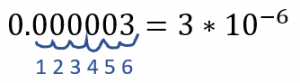
A polynomial is an equation which is created through the use of two or more algebraic terms. In the example below, each color represents a different term.

Polynomials can be made up of some or all of the following:

• Variables: the letters in the equation
• Constants: In the example above, the constant would be the 11. It’s a number that does not contain any modifiable variables.
• Exponents: These are the numbers that you’ll typically find attached to variables
• Addition, subtraction, multiplication, and division

What isn’t Considered a Polynomial?

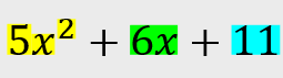
While a polynomial can appear in many different ways, there are some rules about what is not considered a polynomial. A polynomial is NOT:

An equation which contains division by a variable.

An equation that contains negative exponents.

An equation that contains fractional exponents.

An equation that contains radicals.

Evaluating Polynomials

Evaluating polynomials is just like solving any other math problem; make sure to use the order of operations. The order of operations is abbreviated to PEMDAS, which stands for Parentheses, Exponents, Multiplication and Division, and Addition and Subtraction. To start, just plug the value for x or whatever letter you’re working with and then use the order of operations until you get your most simplified answer. Check out the example below:

• Evaluate when
• Step 1: Substitute
  • 
• Step 2: PEMDAS
  • 
• Step 3: PEMDAS
  • 
• Step 4: PEMDAS
  • 

Adding Polynomials

When adding polynomials, keep in mind that you can only add together like terms. The like terms are highlighted in different colors in the example below. Don’t be intimidated by the parentheses when adding – just add like you normally would.

Subtracting Polynomials

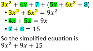
Just like when adding polynomials, only like terms can be subtracted from one another. However, in this case, you do need to keep the parentheses in mind because of the minus side to the left of the second polynomial. Treat the minus sign like a -1, as if you were about to multiply everything in the parentheses by -1. This means that everything that was once positive will be negative and vice versa.

Polynomials with Two Variables

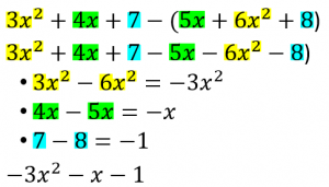
Don’t get distracted by the new variable! The rules from before still apply. Just be sure to separate each type of number by the base and then simplify.

Multiplying Monomials

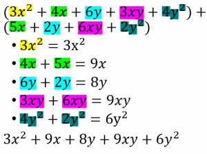
When working in equations that involve variables, multiplying two of the same variable results in an “addition” of exponents. For equations that simply have an “x” or “y,” imagine there’s a 1 exponent above it.

Multiplying Monomials by Polynomials

When multiplying monomials by polynomials, it’s important to multiply the monomial term by every term within the polynomial.

Using FOIL

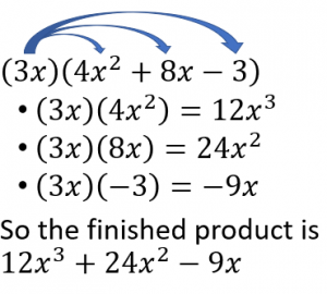
When multiplying two different polynomials, remember to FOIL. First, multiply the two First variables in each polynomial. Then, multiply the Outside variables together. Next, multiply the Inside variables. Finally, multiply the Last variable of each polynomial.

Multiplying Binomials

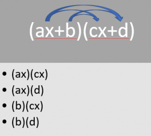
When multiplying binomials, it’s important to remember that each term of the first binomial should be multiplied with each term of the second.

Multiplying Larger Polynomials

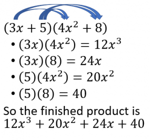
Don’t be intimidated by the added numbers. Just keep in mind that each variable needs to be multiplied by the other variables at some point. With larger polynomials like this one , I typically just go from left to right: .

Check out the example below.

Dividing Polynomials by Monomials

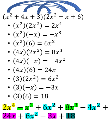
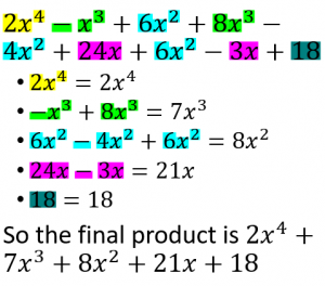
Dividing a Polynomial by a Monomial of often easier when one breaks it up into smaller pieces.

Dividing a Polynomial by Another Polynomial

Solve

Step 1: Rewrite in descending powers and include missing variables ()

Step 2: Long divide, asking yourself “what number multiplied by 2x would equal the number I’m focusing on?”

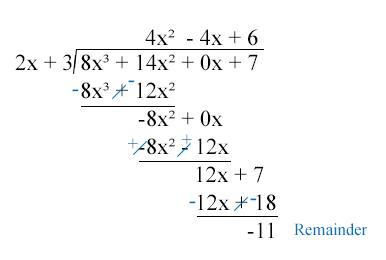
Step 3: Write the remainder out dividing it by the original polynomial

Thus,

This chapter was originally posted to the Math Support Center blog at the University of Baltimore on September 13, 2019. 

Finding the Greatest Common Factor (GCF)

Finding the greatest common factor simply involves finding the largest number or term which will fit evenly into each number or term in a list. The way I like to go about this is by breaking each number or term into its smallest parts. Break each number down until you are multiplying together only prime numbers. All the numbers that they have in common should then be multiplied back up to create the GCF.

This is what it would look like in a list of numbers:

• 
• 
• The greatest common factor is .

And this is what it would look like in a list of terms:

• 
• 
• 
• The greatest common factor is

Sometimes, you will have to factor out the GCF in a function. In this case, treat each term like an individual and follow the instructions mentioned above. Then, whatever the GCF is, divide each term by that GCF, rewrite the function, and make sure to place the GCF outside of a parenthesis which contains the new function.

• 
  • 
  • ; 2 is the greatest common factor
• The final answer is

Factoring by Grouping

• Step 1: Group the terms in two groups of two terms so that each group has a common factor.
• Step 2: Factor out the GCF from each group.
• Step 3: If there is a common binomial factor, factor it out.
• Step 4: If not, rearrange the terms and try these steps again.
• Step 5: Make sure to check your work by multiplying (FOIL-ing) your answer to see if you can get back to the original problem.

Factoring Trinomials of the Form

Sometimes trinomials can be factored into two binomials. It helps to make a chart in order to find the correct pairs of numbers. The pairs of numbers to go into (x+_)(x+_) depend on whether the sum of a pair of factors for the third term is equal to the number presented in the second term.

Factoring Trinomials of the Form

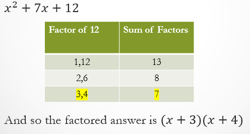
Step 1: Split the first term to and .

Step 2: Find all possible factors of the third term.

• or

Step 3: Test Factors. This first one creates the wrong middle number.

This one also doesn’t work. Just keep testing. Sometimes, you will try everything and it still doesn’t quite work. Try splitting ax differently. In this case, 3 can only be split into 3 and 1, but if you’re working with 6, for example, you could try splitting it into 6 and 1 or 2 and 3.

Step 4: Finally, this set works. Make sure to check your work by FOIL-ing.

Factoring Out the GCF with Polynomials

Sometimes before we can even begin to factor a polynomial, we have the ability to factor out a common factor of all 3 terms. In the example below, notice all the numbers have a GCF of , we can start by factoring it out.

From there, we can continue to factor as we normally would.

Factoring Trinomials of the Form by Grouping

We can also use the grouping method for trinomials. Take the example problem below.

We can rewrite this so that there is an even number of terms, as shown here:

We want to find a factor of 24 (because 2 from the first term multiplied by 12 of the third term) that also adds up to 11.

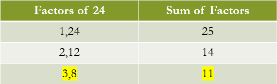
Now that we have our middle numbers, we can group.

Now we’ll factor out the greatest common factors within each group. It looks like we have a common binomial in each group.

So our end product is:

Factoring Perfect Square Trinomials and the Difference of Two Squares

Decide whether is a perfect square trinomial

Two terms and are squares

Twice the product of and is the final term of the trinomial

Thus, is a perfect square trinomial

This means that it can easily be factored to

Factoring the Difference of Two Squares

When both terms in a binomial are squares (meaning that they are a variable which includes a square or a number which can be evenly square-rooted) and the signs of the terms are different, one can use the following equation to factor it:

For example,

Solving Quadratic Equations by Factoring

Factoring can also be used to solve quadratic equations, like so:

• 
• 
• , and so
• , and so

So the solutions to this quadratic equation are 11 and -2.

If the equation has a degree greater than two, it can be solved by factoring and then using the method above.

• 
• 
• 
• , means
• , means
• , means

So the solutions are 0, 2, and -2.

This chapter was originally posted to the Math Support Center blog at the University of Baltimore on September 25, 2019.

What is a Rational Expression?

A rational number is a number that can be written as a quotient of integers. In other words, it’s any number that can create a nice and neat fraction. A rational expression is also a quotient, it’s just made up of polynomials. A rational expression can be written in the form P/Q. For example:

or or

Evaluating Rational Expressions

Rational expressions have different numerical values depending on what values replace the variables. For example:

If then

If then

Identifying When a Rational Expression is Undefined

When the denominator of a rational expression is 0, then it is undefined. There are some equations in which the denominator is sometimes 0 and some in which the denominator is never 0. Take the following equation as an example.

When we set to equal 0, we find that when is 3, the denominator is 0. So when is 3, the rational expression is undefined.

The denominator of the above equation is never 0, and so it is never undefined.

Sometimes you will need to factor the denominator to find the variables which make it undefined, like in the following example.

and

So when equals 2 or 1, the expression is undefined.

Simplifying Rational Expressions

Sometimes a fraction made of polynomials can be simplified. This can be done by taking out the greatest common factor, like in the example below.

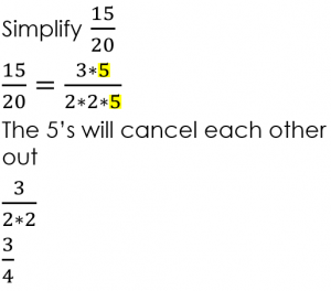
This may also be done by factoring the polynomials in both the numerator and denominator.

Multiplying Rational Expressions

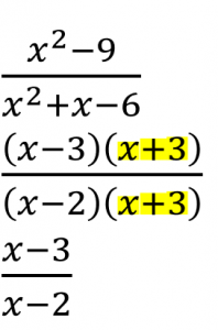
Multiplying rational expressions follow the same rules as multiplying other kinds of fractions. The numerator of one fraction is multiplied by the numerator of the other, and the denominator of one fraction is multiplied by the other.

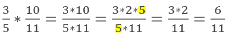
This goes for polynomials as well. Just be sure to FOIL when necessary.

Dividing Rational Expressions

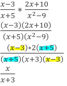
Remember that dividing fractions is the same thing as flipping the second fraction and multiplying.

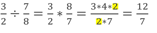
This is also true for polynomials. Again, don’t forget to FOIL when necessary.

Adding and Subtracting Rational Expressions with the Same Denominator

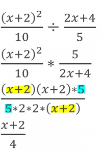
When adding and subtracting with rational expressions that have the same denominator, all you have to worry about is adding and subtracting what’s in the numerator.

This is true for any kind of term that may be in the numerator or denominator.

or

Finding the Least Common Denominator

Finding the least common denominator involves breaking each number up into its smallest variables and seeing how those numbers compare so that the smallest number that they both fit into appears. Take a look at the example below. 8 can be broken up into 2*2*2 and 6 can be broken up into 2*3. We need a number that satisfies the need for all of these numbers, even if a few overlap. The solution to this is 2*2*2*3. It incorporates the 8’s need to have 3 2’s and the 6’s need to have a 2 and a 3. 2*2*2*3 = 24 so our LCD is 24.

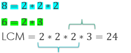
This also works with variables. We’re working with 5x and 15x^2. We need to find a number that fulfills the need of a 5 and an x as well as a 5, a 3, and 2 x’s. The equation 5*x*x*3 fulfills all of those needs. So our LCD is 15x^2.

Writing Equivalent Rational Expressions

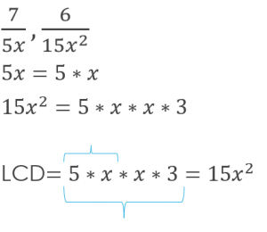
When writing equivalent rational expressions, we are, in a sense, multiplying an expression of 1.

This is useful for when we want to translate one equation to keep the same value but use a different denominator.

In this case, we have to ask ourselves, “what can I multiply by in order to get ?”

Adding and Subtracting Rational Expressions with Different Denominators

Find the LCD and then multiply one rational expression by what’s missing from it to get that LCD in the denominator. Make sure to do this with the other fraction, if necessary, so that in the end, both fractions have the same denominator – the LCD.

Solving Equations Containing Rational Expressions

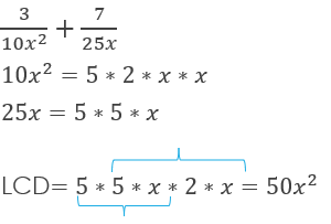
Sometimes, you will be asked to solve for a missing variable when there are equations containing rational expressions. I recommend doing what is needed so that the denominators of all the numbers are eliminated and you can work with whole numbers again.

Another, more complex example would be:

This chapter was originally posted to the Math Support Center blog at the University of Baltimore on October 7, 2019.

Solving Problems by Inductive Reasoning

Before we can talk about how to use inductive reasoning, we need to define it and distinguish it from deductive reasoning.

Inductive reasoning is when one makes generalizations based on repeated observations of specific examples. For instance, if I have only ever had mean math teachers, I might draw the conclusion that all math teachers are mean. Because I witnessed multiple instances of mean math teachers and only mean math teachers, I’ve drawn this conclusion. That being said, one of the downfalls of inductive reasoning is that it only takes meeting one nice math teacher for my original conclusion to be proven false. This is called a counterexample. Since inductive reasoning can so easily be proven false with one counterexample, we don’t say that a conclusion drawn from inductive reasoning is the absolute truth unless we can also prove it using deductive reasoning. With inductive reasoning, we can never be sure that what is true in a specific case will be true in general, but it is a way of making an educated guess.

Deductive reasoning depends on a hypothesis that is considered to be true. In other words, if X = Y and Y = Z, then we can deduce that X = Z. An example of this might be that if we know for a fact that all dogs are good, and Lucky is a dog, then we can deduce that Lucky is good.

Strategies for Problem Solving

No matter what tool you use to solve a problem, there is a method for going about solving the problem.

1. Understand the Problem: You may need to read a problem several times before you can conceptualize it. Don’t become frustrated, and take a walk if you need to. It might take some time to click.
2. Devise a Plan: There may be more than one way to solve the problem. Find the way which is most comfortable for you or the most practical.
3. Carry Out the Plan: Try it out. You may need to adjust your plan if you run into roadblocks or dead ends.
4. Look Back and Check: Make sure your answer gives sense given the context.

There are several different ways one might go about solving a problem. Here are a few:

• Tables and Charts: Sometimes you’ll be working with a lot of data or computing a problem with a lot of different steps. It may be best to keep it organized in a table or chart so you can refer back to previous work later.
• Working Backward: Sometimes you’ll be given a word problem where they describe a series of algebraic functions that took place and then what the end result is. Sometimes you’ll have to work backward chronologically.
• Using Trial and Error: Sometimes you’ll know what mathematical function you need to use but not what number to start with. You may need to use trial and error to get the exact right number.
• Guessing and Checking: Sometimes it will appear that a math problem will have more than one correct answer. Be sure to go back and check your work to determine if some of the answers don’t actually work out.
• Considering a Similar, Simpler Problem: Sometimes you can use the strategy you think you would like to use on a simpler, hypothetical problem first to see if you can find a pattern and apply it to the harder problem.
• Drawing a Sketch: Sometimes—especially with geometrical problems—it’s more helpful to draw a sketch of what is being asked of you.
• Using Common Sense: Be sure to read questions very carefully. Sometimes it will seem like the answer to a question is either too obvious or impossible. There is usually a phrasing of the problem which would lead you to believe that the rules are one way when really it’s describing something else. Pay attention to literal language.

This chapter was originally posted to the Math Support Center blog at the University of Baltimore on November 6, 2019.

Symbols and Terminology

A set is a collection of objects of values that are in this case called elements or members. They can be described using words, lists, or set-builder notation.

• Words: a set of odd numbers less than 6
• Listing: {1,3,5}
• Set-builder notation: {x|x is an odd counting number less than 6}

If a set has no elements, it’s called an empty or null set and its symbol is Ø. Make sure not to write this as {Ø}, because that is technically incorrect.

It is important to make sure that a set is well-defined, meaning that there’s no room for subjective interpretation about whether something belongs in a set or not. An example of a well-defined set is a set of all numbers between 1 and 10. We can say for sure that 5 belongs and 13 doesn’t. A set that is not well defined is a set of all numbers that are aesthetically pleasing. It’s not clear what would define aesthetically pleasing so we’re unsure about whether 5 or 13 would fit.

The symbols ∈ and ∉ are used to describe whether something is or isn’t an element of a set. Going back to our example of all numbers between 1-10 (we’ll name this set A) we can say that 5 ∈ A while 13 ∉ A.

Important Definitions for Sets

Here are some important definitions before moving forward:

• Natural numbers or Counting numbers are all integers starting at 1: {1, 2, 3, 4,…}
• Whole numbers are all integers starting at 0: {0, 1, 2, 3, 4…}
• Integers are all whole numbers from -∞ to ∞: {… -3, -2, -1, 0, 1, 2, 3…}
• Rational numbers are numbers that can be created by dividing two integers (like 1/2 or 9/10 or 4/1).
• Real Numbers are any number that isn’t imaginary, so the typical integer, fraction, or decimal we’re used to. An imaginary number is when a negative number is square rooted (√-1)
• Irrational Numbers are decimals that can’t be expressed as the fraction of two integers. The square root of 2 would be an example of this because the decimals are ongoing and there is no discernible pattern to the decimals.
• A cardinal number is the number of elements in a set and it is written as n(A) and spoken as “n of A.” So if I was given set Z = {1, 5, 7, 2, 9, 10}, I would say n(Z) is 6.
• A finite set is a set that has a whole number as its cardinal number. So we could technically count how many elements are in a set.
• An infinite set is a set where the number of elements is infinite and we couldn’t possibly count them.
• Two sets are equal if two conditions are met: (1) every element of the first set is an element of the second set and (2) if every element of the second set is an element of the first one. That being said, it does not matter if the elements are written in a different order ({a, b, c, d} = {a, c, d, b}) and repeating elements doesn’t add a new element ({a, b, a, c, d, d} = {a, b, c, d}).

Venn Diagrams and Subsets

The universe in which we are working, or the area that we’re concerned within a set, is called the universal set. This consists of everything in the wider set. Venn diagrams are often used to discuss commonalities and differences between sets in the universal set. The universal set is everything within the rectangle encompassing the Venn diagram including the Venn diagram itself. The Venn diagram is made up of sets within U and can overlap. Set A is everything in circle A, set B is everything in circle B, and where they overlap are all the elements that they have in common.

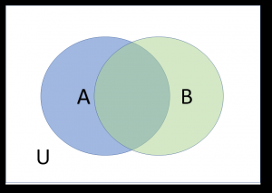
Complements of a set are everything that a set is not. The complement of A is A’ (spoken as A prime) and it includes everything in U except what is included in A.

Subsets of a Set

A subset is any set that is also part of another set. For example, if U = {1, 2, 3, 4, 5} and A = {1, 4, 5}, then we would say that A is a subset of U. This is denoted like this: A ⊆ U. If B = {1, 2, 4, 7}, because 7 is not part of U, we would say B is not a subset of U, also denoted like this: B ⊄ U.

There are different kinds of subsets. Any subset can be called a subset, but some can be described as a proper subset. A proper subset is a subset that has elements of a set but not exactly all of the elements in that set. For example, if set Y = {1, 2, 3} and Z = {1, 2, 3, 4}, then we could say that Y is a subset of Z and we could also say that Y is a proper subset of Z because it does not include all of the elements of Z. This is written as such: Y ⊂ Z.

Sometimes you will be asked to calculate how many subsets exist within a set. This can be calculated using powers of 2. For example, if I have the set {1, 4, 6, 2, 7}, I can see that there are 5 elements in the set. I make that 5 an exponent of 2 (2^5) to calculate how many subsets are possible: 32. To calculate the number of proper subsets, the equation is (2^n) – 1.

Set Operations

An intersection of sets is the elements of two sets that they have in common. For example, {1, 4, 5} ∩ {6, 9, 5} = {5}. Put in other words, A ∩ B = {x|x ∈ A and x ∈ B}. If two sets have no elements in common, they are called disjointed sets and written as such: A ∩ B = ø. A union of sets is the set of all elements belonging to either set one or set two, written as such: A ∪ B = {x|x ∈ A or x ∈ B}. A difference of sets is the set of all elements of the first set and not the second. For example, if set A is {1, 2, 3, 4, 5, 6} and B is {1, 3, 5}, then the difference would be {2, 4,6}. In other words, A – B = {x|x ∈ A and x ∉ B}.

When elements are placed in {braces}, it doesn’t matter in what order they are listed. When elements are placed in (parentheses), it’s called an ordered pair and it does matter what order they are listed in. In other words (a,b) ≠ (b,a). In the ordered pair (a,b), a is the first component and b is the second component.

A cartesian product of sets is a way of creating a set of ordered pairs. It’s written like A X B and when presented with a problem asking you to find cartesian products, you have to create ordered pairs with each number in each set in the order that the notation dictates. For example, if A = {1, 2, 3} and B = {8, 9}, and you were asked to find A X B, then the answer would be {(1,8), (1,9), (2,8), (2,9), (3,8), (3,9)}. If you were asked to find B X A, the answer would be {(8,1), (8,2), (8,3), (9,1), (9,2), (9,3)}. The cardinal number of a cartesian product is going to be the cardinal number of set 1 times the cardinal number of set 2, or n(A) x n(B).

This chapter was originally posted to the Math Support Center blog at the University of Baltimore on November 11, 2019.